3.1: Matrix Transformations

\(\usepackage{macros} \newcommand{\lt}{<} \newcommand{\gt}{>} \newcommand{\amp}{&} \)

Objectives

1. Learn to view a matrix geometrically as a function.
2. Learn examples of matrix transformations: reflection, dilation, rotation, shear, projection.
3. Understand the vocabulary surrounding transformations: domain, codomain, range.
4. Understand the domain, codomain, and range of a matrix transformation.
5. Pictures: common matrix transformations.
6. Vocabulary words: transformation / function, domain, codomain, range, identity transformation, matrix transformation.

In this section we learn to understand matrices geometrically as functions, or transformations. We briefly discuss transformations in general, then specialize to matrix transformations, which are transformations that come from matrices.

Matrices as Functions

Informally, a function is a rule that accepts inputs and produces outputs. For instance, \(f(x) = x^2\) is a function that accepts one number \(x\) as its input, and outputs the square of that number: \(f(2) = 4\). In this subsection, we interpret matrices as functions.

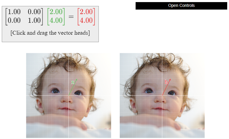
Let \(A\) be a matrix with \(m\) rows and \(n\) columns. Consider the matrix equation \(b=Ax\) (we write it this way instead of \(Ax=b\) to remind the reader of the notation \(y=f(x)\)). If we vary \(x\text{,}\) then \(b\) will also vary; in this way, we think of \(A\) as a function with independent variable \(x\) and dependent variable \(b\).

• The independent variable (the input) is \(x\text{,}\) which is a vector in \(\mathbb{R}^n \).
• The dependent variable (the output) is \(b\text{,}\) which is a vector in \(\mathbb{R}^m \).

The set of all possible output vectors are the vectors \(b\) such that \(Ax=b\) has some solution; this is the same as the column space of \(A\) by Note 2.3.6 in Section 2.3.

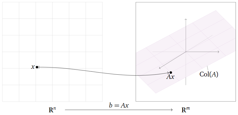
Figure \(\PageIndex{1}\)

Example \(\PageIndex{1}\): Interactive: A \(2\times 3\) matrix

Figure \(\PageIndex{2}\): A picture of a \(2\times 3\) matrix, regarded as a function. The input vector is \(x\text{,}\) which is a vector in \(\mathbb{R}^3 \text{,}\) and the output vector is \(b=Ax\text{,}\) which is a vector in \(\mathbb{R}^2 \). The violet line on the right is the column space; as you vary \(x\text{,}\) the output \(b\) is constrained to lie on this line.

Example \(\PageIndex{2}\): Interactive: A \(3\times 2\) matrix

Figure \(\PageIndex{3}\): A picture of a \(3\times 2\) matrix, regarded as a function. The input vector is \(x\text{,}\) which is a vector in \(\mathbb{R}^2 \text{,}\) and the output vector is \(b=Ax\text{,}\) which is a vector in \(\mathbb{R}^3 \). The violet plane on the right is the column space; as you vary \(x\text{,}\) the output \(b\) is constrained to lie on this plane.

Example \(\PageIndex{3}\): Projection onto the \(xy\)-plane

Let

\[A=\left(\begin{array}{ccc}1&0&0\\0&1&0\\0&0&0\end{array}\right).\nonumber\]

Describe the function \(b=Ax\) geometrically.

Solution

In the equation \(Ax=b\text{,}\) the input vector \(x\) and the output vector \(b\) are both in \(\mathbb{R}^3 \). First we multiply \(A\) by a vector to see what it does:

\[A\left(\begin{array}{c}x\\y\\z\end{array}\right)=\left(\begin{array}{ccc}1&0&0\\0&1&0\\0&0&0\end{array}\right)\:\left(\begin{array}{c}x\\y\\z\end{array}\right)=\left(\begin{array}{c}x\\y\\0\end{array}\right).\nonumber\]

Multiplication by \(A\) simply sets the \(z\)-coordinate equal to zero: it projects vertically onto the \(xy\)-plane. 

Figure \(\PageIndex{4}\)

Figure \(\PageIndex{5}\): Multiplication by the matrix \(A\) projects a vector onto the \(xy\)-plane. Move the input vector \(x\) to see how the output vector \(b\) changes.

Example \(\PageIndex{4}\): Reflection

Let

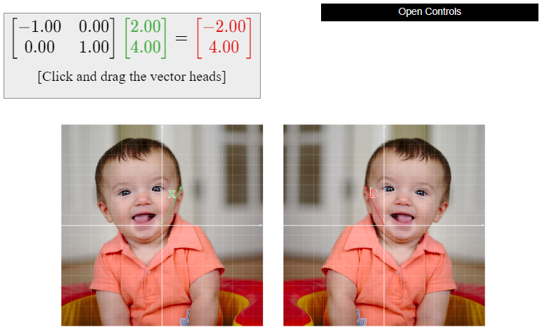
\[A=\left(\begin{array}{cc}-1&0\\0&1\end{array}\right).\nonumber\]

Describe the function \(b=Ax\) geometrically.

Solution

In the equation \(Ax=b\text{,}\) the input vector \(x\) and the output vector \(b\) are both in \(\mathbb{R}^2 \). First we multiply \(A\) by a vector to see what it does:

\[A\left(\begin{array}{c}x\\y\end{array}\right)=\left(\begin{array}{cc}-1&0\\0&1\end{array}\right)\:\left(\begin{array}{c}x\\y\end{array}\right)=\left(\begin{array}{c}-x\\y\end{array}\right).\nonumber\]

Multiplication by \(A\) negates the \(x\)-coordinate: it reflects over the \(y\)-axis.

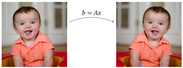
Figure \(\PageIndex{6}\)

Figure \(\PageIndex{7}\): Multiplication by the matrix \(A\) reflects over the \(y\)-axis. Move the input vector \(x\) to see how the output vector \(b\) changes.

Example \(\PageIndex{5}\): Dilation

Let

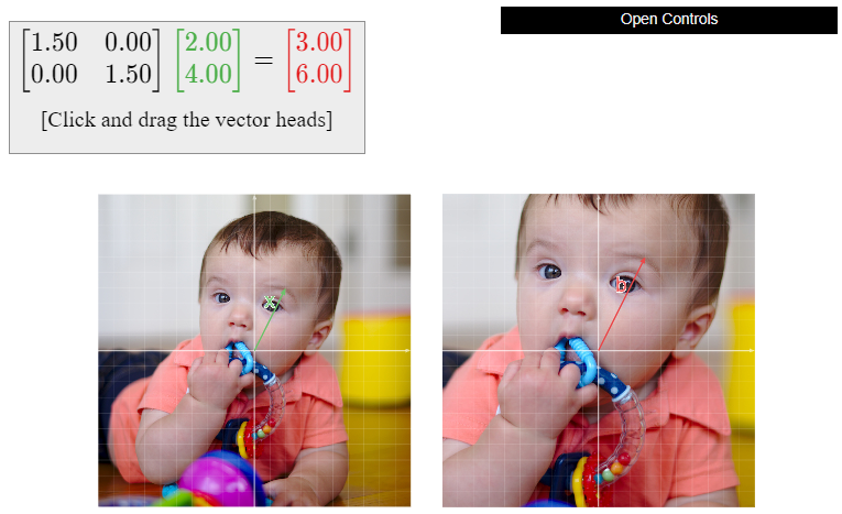
\[A=\left(\begin{array}{cc}1.5&0\\0&1.5\end{array}\right).\nonumber\]

Describe the function \(b=Ax\) geometrically.

Solution

In the equation \(Ax=b\text{,}\) the input vector \(x\) and the output vector \(b\) are both in \(\mathbb{R}^2 \). First we multiply \(A\) by a vector to see what it does:

\[A\left(\begin{array}{c}x\\y\end{array}\right)=\left(\begin{array}{cc}1.5&0\\0&1.5\end{array}\right)\:\left(\begin{array}{c}x\\y\end{array}\right)=\left(\begin{array}{c}1.5x\\1.5y\end{array}\right)=1.5\left(\begin{array}{c}x\\y\end{array}\right).\nonumber\]

Multiplication by \(A\) is the same as scalar multiplication by \(1.5\text{:}\) it scales or dilates the plane by a factor of \(1.5\).

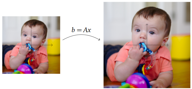
Figure \(\PageIndex{8}\)

Figure \(\PageIndex{9}\): Multiplication by the matrix \(A\) dilates the plane by a factor of \(1.5\). Move the input vector \(x\) to see how the output vector \(b\) changes.

Example \(\PageIndex{6}\): Identity

Let

\[A=\left(\begin{array}{cc}1&0\\0&1\end{array}\right).\nonumber\]

Describe the function \(b=Ax\) geometrically.

Solution

In the equation \(Ax=b\text{,}\) the input vector \(x\) and the output vector \(b\) are both in \(\mathbb{R}^2 \). First we multiply \(A\) by a vector to see what it does:

\[A\left(\begin{array}{c}x\\y\end{array}\right)=\left(\begin{array}{cc}1&0\\0&1\end{array}\right)\:\left(\begin{array}{c}x\\y\end{array}\right)=\left(\begin{array}{c}x\\y\end{array}\right).\nonumber\]

Multiplication by \(A\) does not change the input vector at all: it is the identity transformation which does nothing. 

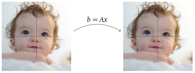
Figure \(\PageIndex{10}\)

Figure \(\PageIndex{11}\): Multiplication by the matrix \(A\) does not move the vector \(x\text{:}\) that is, \(b=Ax=x\). Move the input vector \(x\) to see how the output vector \(b\) changes.

Example \(\PageIndex{7}\): Rotation

Let

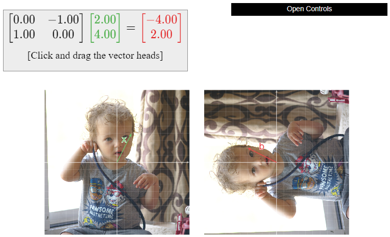
\[A=\left(\begin{array}{cc}0&-1\\1&0\end{array}\right).\nonumber\]

Describe the function \(b=Ax\) geometrically.

Solution

In the equation \(Ax=b\text{,}\) the input vector \(x\) and the output vector \(b\) are both in \(\mathbb{R}^2 \). First we multiply \(A\) by a vector to see what it does:

\[A\left(\begin{array}{c}x\\y\end{array}\right)=\left(\begin{array}{cc}0&-1\\1&0\end{array}\right)\:\left(\begin{array}{c}x\\y\end{array}\right)=\left(\begin{array}{c}-y\\x\end{array}\right).\nonumber\]

We substitute a few test points in order to understand the geometry of the transformation:

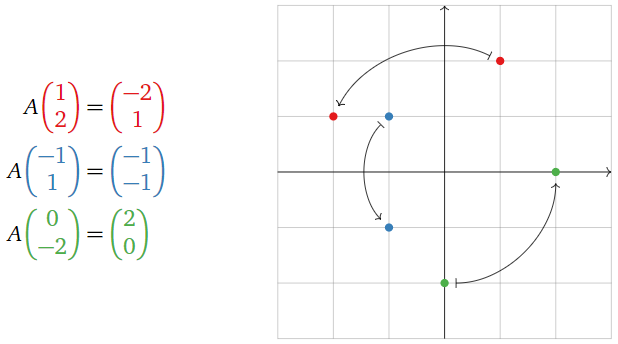
Figure \(\PageIndex{12}\)

Multiplication by \(A\) is counterclockwise rotation by \(90^\circ\).

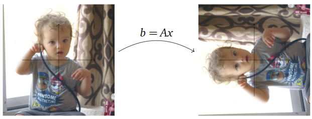
Figure \(\PageIndex{13}\)

Figure \(\PageIndex{14}\): Multiplication by the matrix \(A\) rotates the vector \(x\) counterclockwise by \(90^\circ\). Move the input vector \(x\) to see how the output vector \(b\) changes.

Example \(\PageIndex{8}\): Shear

Let

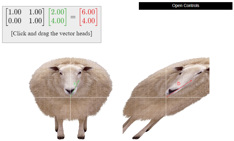
\[A=\left(\begin{array}{cc}1&1\\0&1\end{array}\right).\nonumber\]

Describe the function \(b=Ax\) geometrically.

Solution

In the equation \(Ax=b\text{,}\) the input vector \(x\) and the output vector \(b\) are both in \(\mathbb{R}^2 \). First we multiply \(A\) by a vector to see what it does:

\[A\left(\begin{array}{c}x\\y\end{array}\right)=\left(\begin{array}{cc}1&1\\0&1\end{array}\right)\:\left(\begin{array}{c}x\\y\end{array}\right)=\left(\begin{array}{c}x+y\\y\end{array}\right).\nonumber\]

Multiplication by \(A\) adds the \(y\)-coordinate to the \(x\)-coordinate; this is called a shear in the \(x\)-direction. 

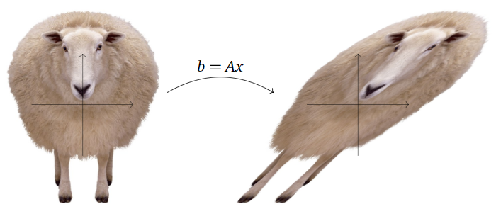
Figure \(\PageIndex{15}\)

Figure \(\PageIndex{16}\): Multiplication by the matrix \(A\) adds the \(y\)-coordinate to the \(x\)-coordinate. Move the input vector \(x\) to see how the output vector \(b\) changes.

Transformations

At this point it is convenient to fix our ideas and terminology regarding functions, which we will call transformations in this book. This allows us to systematize our discussion of matrices as functions.

Definition \(\PageIndex{1}\): Transformation

A transformation from \(\mathbb{R}^n \) to \(\mathbb{R}^m \) is a rule \(T\) that assigns to each vector \(x\) in \(\mathbb{R}^n \) a vector \(T(x)\) in \(\mathbb{R}^m \).

• \(\mathbb{R}^n \) is called the domain of \(T\).
• \(\mathbb{R}^m \) is called the codomain of \(T\).
• For \(x\) in \(\mathbb{R}^n \text{,}\) the vector \(T(x)\) in \(\mathbb{R}^m \) is the image of \(x\) under \(T\).
• The set of all images \(\{T(x)\mid x\text{ in }\mathbb{R}^n \}\) is the range of \(T\).

The notation \(T\colon\mathbb{R}^n \to \mathbb{R}^m \) means “\(T\) is a transformation from \(\mathbb{R}^n \) to \(\mathbb{R}^m \).”

It may help to think of \(T\) as a “machine” that takes \(x\) as an input, and gives you \(T(x)\) as the output.

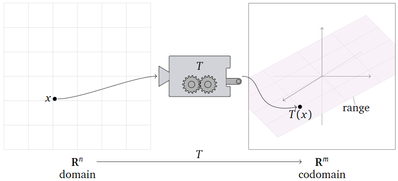
Figure \(\PageIndex{17}\)

The points of the domain \(\mathbb{R}^n \) are the inputs of \(T\text{:}\) this simply means that it makes sense to evaluate \(T\) on vectors with \(n\) entries, i.e., lists of \(n\) numbers. Likewise, the points of the codomain \(\mathbb{R}^m \) are the outputs of \(T\text{:}\) this means that the result of evaluating \(T\) is always a vector with \(m\) entries.

The range of \(T\) is the set of all vectors in the codomain that actually arise as outputs of the function \(T\text{,}\) for some input. In other words, the range is all vectors \(b\) in the codomain such that \(T(x)=b\) has a solution \(x\) in the domain.

Example \(\PageIndex{9}\): A Function of one variable

Most of the functions you may have seen previously have domain and codomain equal to \(\mathbb{R} = \mathbb{R}^1\). For example,

\[\sin :\mathbb{R}\to\mathbb{R}\quad\sin(x)=\left(\begin{array}{l}\text{the length of the opposite} \\ \text{edge over the hypotenuse of} \\ \text{a right triangle with angle }x \\ \text{in radians}\end{array}\right).\nonumber\]

Notice that we have defined \(\sin\) by a rule: a function is defined by specifying what the output of the function is for any possible input.

You may be used to thinking of such functions in terms of their graphs:

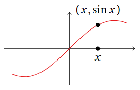
Figure \(\PageIndex{18}\)

In this case, the horizontal axis is the domain, and the vertical axis is the codomain. This is useful when the domain and codomain are \(\mathbb{R}\text{,}\) but it is hard to do when, for instance, the domain is \(\mathbb{R}^2 \) and the codomain is \(\mathbb{R}^3 \). The graph of such a function is a subset of \(\mathbb{R}^5\text{,}\) which is difficult to visualize. For this reason, we will rarely graph a transformation.

Note that the range of \(\sin\) is the interval \([-1,1]\text{:}\) this is the set of all possible outputs of the \(\sin\) function.

Example \(\PageIndex{10}\): Functions of several variables

Here is an example of a function from \(\mathbb{R}^2 \) to \(\mathbb{R}^3 \text{:}\)

\[f\left(\begin{array}{c}x\\y\end{array}\right)=\left(\begin{array}{c}x+y\\ \cos(y) \\y-x^{2}\end{array}\right).\nonumber\]

The inputs of \(f\) each have two entries, and the outputs have three entries. In this case, we have defined \(f\) by a formula, so we evaluate \(f\) by substituting values for the variables:

\[f\left(\begin{array}{c}2\\3\end{array}\right)=\left(\begin{array}{c}2+3 \\ \cos(3) \\ 3-2^2\end{array}\right)=\left(\begin{array}{c}5\\ \cos(3)\\-1\end{array}\right).\nonumber\]

Here is an example of a function from \(\mathbb{R}^3 \) to \(\mathbb{R}^3 \text{:}\)

\[f(v)=\left(\begin{array}{c}\text{the counterclockwise rotation} \\ \text{of }v\text{ by and angle of }42^\circ \text{ about} \\ \text{ the }z\text{-axis}\end{array}\right).\nonumber\]

In other words, \(f\) takes a vector with three entries, then rotates it; hence the ouput of \(f\) also has three entries. In this case, we have defined \(f\) by a geometric rule.

Definition \(\PageIndex{2}\): Identity Transformation

The identity transformation \(\text{Id}_{\mathbb{R}^n }\colon\mathbb{R}^n \to\mathbb{R}^n \) is the transformation defined by the rule

\[ \text{Id}_{\mathbb{R}^n }(x) = x \qquad\text{for all $x$ in $\mathbb{R}^n $}. \nonumber \]

In other words, the identity transformation does not move its input vector: the output is the same as the input. Its domain and codomain are both \(\mathbb{R}^n \text{,}\) and its range is \(\mathbb{R}^n \) as well, since every vector in \(\mathbb{R}^n \) is the output of itself.

Example \(\PageIndex{11}\): A real-word transformation: robotics

The definition of transformation and its associated vocabulary may seem quite abstract, but transformations are extremely common in real life. Here is an example from the fields of robotics and computer graphics.

Suppose you are building a robot arm with three joints that can move its hand around a plane, as in the following picture.

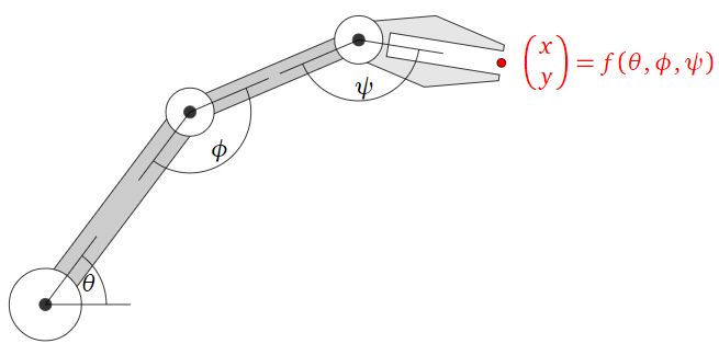
Figure \(\PageIndex{19}\)

Define a transformation \(f\colon\mathbb{R}^3 \to\mathbb{R}^2 \) as follows: \(f(\theta,\phi,\psi)\) is the \((x,y)\) position of the hand when the joints are rotated by angles \(\theta, \phi, \psi\text{,}\) respectively. Evaluating \(f\) tells you where the hand will be on the plane when the joints are set at the given angles.

It is relatively straightforward to find a formula for \(f(\theta,\phi,\psi)\) using some basic trigonometry. If you want the robot to fetch your coffee cup, however, you have to find the angles \(\theta,\phi,\psi\) that will put the hand at the position of your beverage. It is not at all obvious how to do this, and it is not even clear if the answer is unique! You can ask yourself: “which positions on the table can my robot arm reach?” or “what is the arm’s range of motion?” This is the same as asking: “what is the range of \(f\text{?}\)”

Unfortunately, this kind of function does not come from a matrix, so one cannot use linear algebra to answer these kinds of questions. In fact, these functions are rather complicated; their study is the subject of inverse kinematics.

Matrix Transformations

Now we specialize the general notions and vocabulary from the previous Subsection Transformations to the functions defined by matrices that we considered in the first Subsection Matrices as Functions.

Definition \(\PageIndex{3}\): Matrix Transformation

Let \(A\) be an \(m\times n\) matrix. The matrix transformation associated to \(A\) is the transformation

\[ T\colon \mathbb{R}^n \to \mathbb{R}^m \quad\text{defined by}\quad T(x) = Ax. \nonumber \]

This is the transformation that takes a vector \(x\) in \(\mathbb{R}^n \) to the vector \(Ax\) in \(\mathbb{R}^m \).

If \(A\) has \(n\) columns, then it only makes sense to multiply \(A\) by vectors with \(n\) entries. This is why the domain of \(T(x)=Ax\) is \(\mathbb{R}^n \). If \(A\) has \(n\) rows, then \(Ax\) has \(m\) entries for any vector \(x\) in \(\mathbb{R}^n \text{;}\) this is why the codomain of \(T(x)=Ax\) is \(\mathbb{R}^m \).

The definition of a matrix transformation \(T\) tells us how to evaluate \(T\) on any given vector: we multiply the input vector by a matrix. For instance, let

\[A=\left(\begin{array}{ccc}1&2&3\\4&5&6\end{array}\right)\nonumber\]

and let \(T(x)=Ax\) be the associated matrix transformation. Then

\[T\left(\begin{array}{c}-1\\-2\\-3\end{array}\right)=A\left(\begin{array}{c}-1\\-2\\-3\end{array}\right)=\left(\begin{array}{ccc}1&2&3\\4&5&6\end{array}\right)\:\left(\begin{array}{c}-1\\-2\\-3\end{array}\right)=\left(\begin{array}{c}-14\\-32\end{array}\right).\nonumber\]

Suppose that \(A\) has columns \(v_1,v_2,\ldots,v_n\). If we multiply \(A\) by a general vector \(x\text{,}\) we get

\[Ax=\left(\begin{array}{cccc}|&|&\quad&| \\ v_1&v&2&\cdots &v_n \\ |&|&\quad &|\end{array}\right)\:\left(\begin{array}{c}x_1\\x_2\\ \vdots \\x_n\end{array}\right)=x_1v_1+x_2v_2+\cdots +x_nv_n.\nonumber\]

This is just a general linear combination of \(v_1,v_2,\ldots,v_n\). Therefore, the outputs of \(T(x) = Ax\) are exactly the linear combinations of the columns of \(A\text{:}\) the range of \(T\) is the column space of \(A\). See Note 2.3.6 in Section 2.3.

Note \(\PageIndex{1}\)

Let \(A\) be an \(m\times n\) matrix, and let \(T(x)=Ax\) be the associated matrix transformation.

• The domain of \(T\) is \(\mathbb{R}^n \text{,}\) where \(n\) is the number of columns of \(A\).
• The codomain of \(T\) is \(\mathbb{R}^m \text{,}\) where \(m\) is the number of rows of \(A\).
• The range of \(T\) is the column space of \(A\).

Example \(\PageIndex{12}\): Interactive: A \(2\times 3\) matrix: reprise

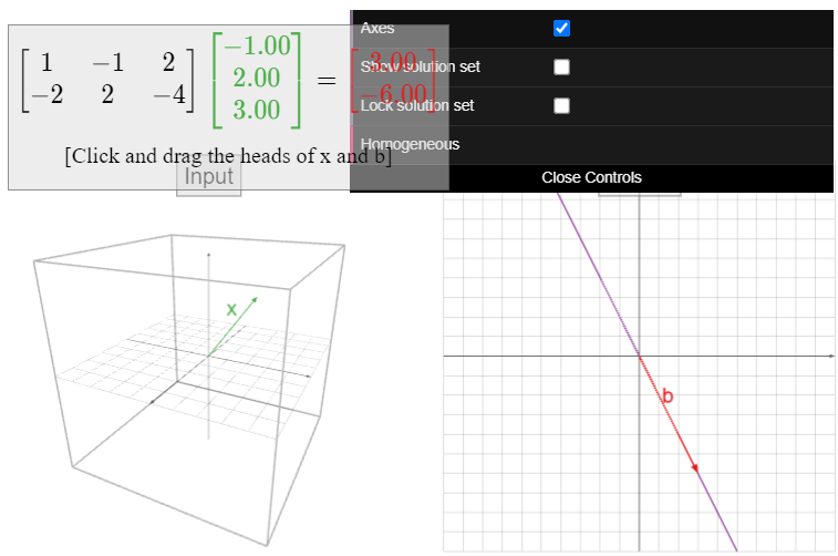
Let

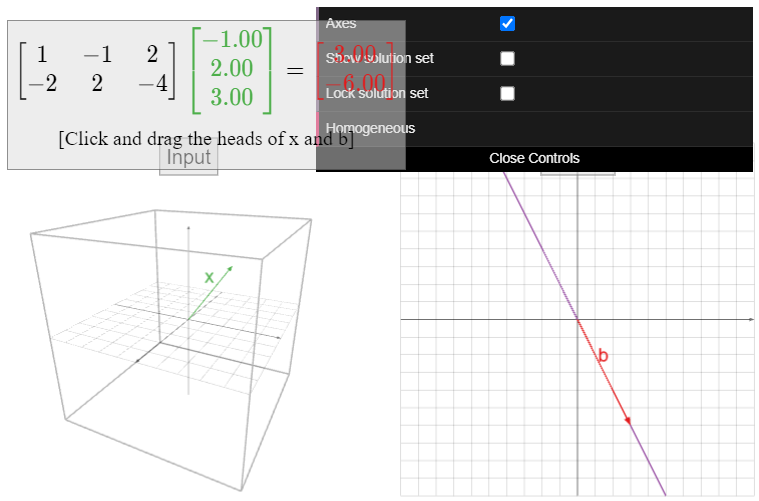
\[A=\left(\begin{array}{c}1&-1&2\\-2&2&4\end{array}\right),\nonumber\]

and define \(T(x) = Ax\). The domain of \(T\) is \(\mathbb{R}^3 \text{,}\) and the codomain is \(\mathbb{R}^2 \). The range of \(T\) is the column space; since all three columns are collinear, the range is a line in \(\mathbb{R}^2 \).

Figure \(\PageIndex{20}\): A picture of the matrix transformation \(T\). The input vector is \(x\text{,}\) which is a vector in \(\mathbb{R}^3 \text{,}\) and the output vector is \(b=T(x)=Ax\text{,}\) which is a vector in \(\mathbb{R}^2 \). The violet line on the right is the range of \(T\text{;}\) as you vary \(x\text{,}\) the output \(b\) is constrained to lie on this line.

Example \(\PageIndex{13}\): Interactive: A \(3\times 2\) matrix: reprise

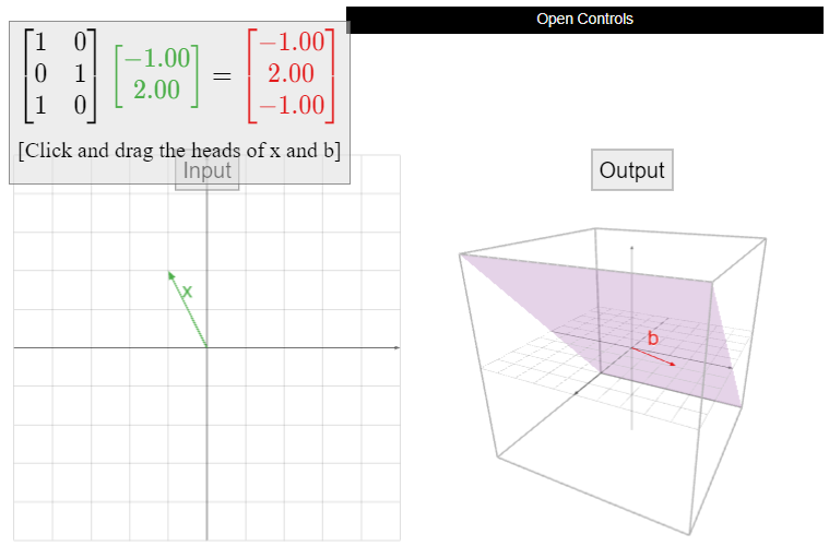
Let

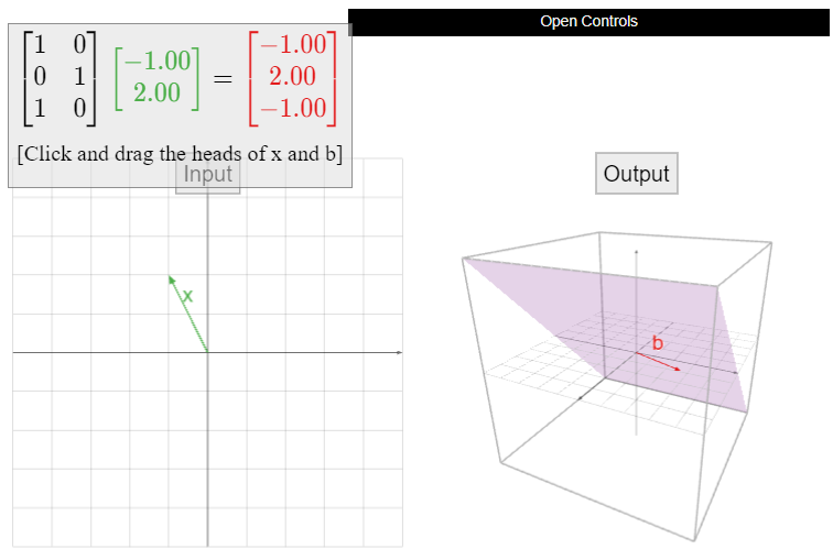
\[A=\left(\begin{array}{cc}1&0\\0&1\\1&0\end{array}\right),\nonumber\]

and define \(T(x) = Ax\). The domain of \(T\) is \(\mathbb{R}^2 \text{,}\) and the codomain is \(\mathbb{R}^3 \). The range of \(T\) is the column space; since \(A\) has two columns which are not collinear, the range is a plane in \(\mathbb{R}^3 \).

Figure \(\PageIndex{21}\): A picture of the matrix transformation \(T\). The input vector is \(x\text{,}\) which is a vector in \(\mathbb{R}^2 \text{,}\) and the output vector is \(b=T(x)=Ax\text{,}\) which is a vector in \(\mathbb{R}^3 \). The violet plane on the right is the range of \(T\text{;}\) as you vary \(x\text{,}\) the output \(b\) is constrained to lie on this plane.

Example \(\PageIndex{14}\): Projection onto the \(xy\)-plane: reprise

Let

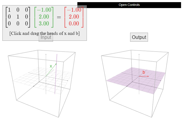
\[A=\left(\begin{array}{ccc}1&0&0\\0&1&0\\0&0&0\end{array}\right),\nonumber\]

and let \(T(x) = Ax\). What are the domain, the codomain, and the range of \(T\text{?}\)

Solution

Geometrically, the transformation \(T\) projects a vector directly “down” onto the \(xy\)-plane in \(\mathbb{R}^3 \).

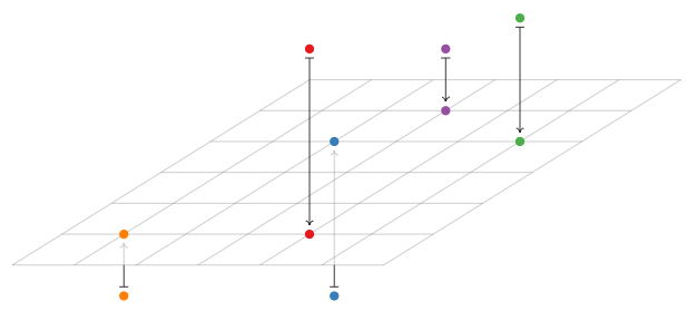
Figure \(\PageIndex{22}\)

The inputs and outputs have three entries, so the domain and codomain are both \(\mathbb{R}^3 \). The possible outputs all lie on the \(xy\)-plane, and every point on the \(xy\)-plane is an output of \(T\) (with itself as the input), so the range of \(T\) is the \(xy\)-plane.

Be careful not to confuse the codomain with the range here. The range is a plane, but it is a plane in \(\mathbb{R}^3 \), so the codomain is still \(\mathbb{R}^3 \). The outputs of \(T\) all have three entries; the last entry is simply always zero.

In the case of an \(n\times n\) square matrix, the domain and codomain of \(T(x) = Ax\) are both \(\mathbb{R}^n \). In this situation, one can regard \(T\) as operating on \(\mathbb{R}^n \text{:}\) it moves the vectors around in the same space.

Example \(\PageIndex{15}\): Matrix transformations of \(\mathbb{R}^2 \)

In the first Subsection Matrices as Functions we discussed the transformations defined by several \(2\times 2\) matrices, namely:

\begin{align*} \text{Reflection:} &\qquad A=\left(\begin{array}{cc}-1&0\\0&1\end{array}\right) \\ \text{Dilation:} &\qquad A=\left(\begin{array}{cc}1.5&0\\0&1.5\end{array}\right) \\ \text{Identity:} &\qquad A=\left(\begin{array}{cc}1&0\\0&1\end{array}\right) \\ \text{Rotation:} &\qquad A=\left(\begin{array}{cc}0&-1\\1&0\end{array}\right) \\ \text{Shear:} &\qquad A=\left(\begin{array}{cc}1&1\\0&1\end{array}\right). \end{align*}

In each case, the associated matrix transformation \(T(x)=Ax\) has domain and codomain equal to \(\mathbb{R}^2 \). The range is also \(\mathbb{R}^2 \text{,}\) as can be seen geometrically (what is the input for a given output?), or using the fact that the columns of \(A\) are not collinear (so they form a basis for \(\mathbb{R}^2 \)).

Example \(\PageIndex{16}\): Questions about a [matrix] transformation

Let

\[A=\left(\begin{array}{cc}1&1\\0&1\\1&1\end{array}\right),\nonumber\]

and let \(T(x)=Ax\text{,}\) so \(T\colon\mathbb{R}^2 \to\mathbb{R}^3 \) is a matrix transformation.

1. Evaluate \(T(u)\) for \(u=\left(\begin{array}{c}3\\4\end{array}\right)\).
2. Let
   \[ b = \left(\begin{array}{c}7\\5\\7\end{array}\right). \nonumber \]
   Find a vector \(v\) in \(\mathbb{R}^2 \) such that \(T(v)=b\). Is there more than one?
3. Does there exist a vector \(w\) in \(\mathbb{R}^3 \) such that there is more than one \(v\) in \(\mathbb{R}^2 \) with \(T(v)=w\text{?}\)
4. Find a vector \(w\) in \(\mathbb{R}^3 \) which is not in the range of \(T\).

Note: all of the above questions are intrinsic to the transformation \(T\text{:}\) they make sense to ask whether or not \(T\) is a matrix transformation. See the next Example \(\PageIndex{17}\). As \(T\) is in fact a matrix transformation, all of these questions will translate into questions about the corresponding matrix \(A\).

Solution

1. We evaluate \(T(u)\) by substituting the definition of \(T\) in terms of matrix multiplication:
   \[T\left(\begin{array}{c}3\\4\end{array}\right)=\left(\begin{array}{cc}1&1\\0&1\\1&1\end{array}\right)\:\left(\begin{array}{c}3\\4\end{array}\right)=\left(\begin{array}{c}7\\4\\7\end{array}\right).\nonumber\]
2. We want to find a vector \(v\) such that \(b = T(v) = Av\). In other words, we want to solve the matrix equation \(Av = b\). We form an augmented matrix and row reduce:
   \[\left(\begin{array}{cc}1&1\\0&1\\1&1\end{array}\right)v=\left(\begin{array}{c}7\\5\\7\end{array}\right) \quad\xrightarrow{\text{augmented matrix}}\quad\left(\begin{array}{cc|c}1&1&7\\0&1&5\\1&1&7\end{array}\right) \quad\xrightarrow{\text{row reduce}}\quad\left(\begin{array}{cc|c}1&0&2\\0&1&5\\0&0&0\end{array}\right).\nonumber\]
   This gives \(x=2\) and \(y=5\text{,}\) so that there is a unique vector
   \[ v = \left(\begin{array}{c}2\\5\end{array}\right) \nonumber \]
   such that \(T(v) = b\).
3. Translation: is there any vector \(w\) in \(\mathbb{R}^3 \) such that the solution set of \(Av=w\) has more than one vector in it? The solution set of \(Ax=w\text{,}\) if non-empty, is a translate of the solution set of \(Av=b\) above, which has one vector in it. See key observation 2.4.3 in Section 2.4. It follows that the solution set of \(Av=w\) can have at most one vector.
4. Translation: find a vector \(w\) such that the matrix equation \(Av=w\) is not consistent. Notice that if we take
   \[ w = \left(\begin{array}{c}1\\2\\3\end{array}\right)\text{,} \nonumber \]
   then the matrix equation \(Av=w\) translates into the system of equations
   \[\left\{\begin{array}{rrrrl}x &+& y &=& 1\\ {}&{}& y &=& 2\\ x &+& y &=& 3,\end{array}\right.\nonumber\]
   which is clearly inconsistent.

Example \(\PageIndex{17}\): Questions about a [non-matrix] transformation

Define a transformation \(T\colon\mathbb{R}^2 \to\mathbb{R}^3 \) by the formula

\[T\left(\begin{array}{c}x\\y\end{array}\right)=\left(\begin{array}{c}\ln(x) \\ \cos(y) \\ \ln(x)\end{array}\right).\nonumber\]

1. Evaluate \(T(u)\) for \(u=\left(\begin{array}{c}1\\ \pi\end{array}\right)\).
2. Let
   \[ b = \left(\begin{array}{c}7\\1\\7\end{array}\right). \nonumber \]
   Find a vector \(v\) in \(\mathbb{R}^2 \) such that \(T(v)=b\). Is there more than one?
3. Does there exist a vector \(w\) in \(\mathbb{R}^3 \) such that there is more than one \(v\) in \(\mathbb{R}^2 \) with \(T(v)=w\text{?}\)
4. Find a vector \(w\) in \(\mathbb{R}^3 \) which is not in the range of \(T\).

Note: we asked (almost) the exact same questions about a matrix transformation in the previous Example \(\PageIndex{16}\). The point of this example is to illustrate the fact that the questions make sense for a transformation that has no hope of coming from a matrix. In this case, these questions do not translate into questions about a matrix; they have to be answered in some other way.

Solution

1. We evaluate \(T(u)\) using the defining formula:
   \[T\left(\begin{array}{c}1\\ \pi\end{array}\right)=\left(\begin{array}{c} \ln(1) \\ \cos(\pi ) \\ \ln(1)\end{array}\right)=\left(\begin{array}{c}0\\-1\\0\end{array}\right).\nonumber\]
2. We have
   \[T\left(\begin{array}{c}e^7 \\ 2\pi n \\ e^7\end{array}\right)=\left(\begin{array}{c}\ln(e^7) \\ \cos (2\pi n) \\ \ln(e^7)\end{array}\right)=\left(\begin{array}{c}7\\1\\7\end{array}\right)\nonumber\]
   for any whole number \(n\). Hence there are infinitely many such vectors.
3. The vector \(b\) from the previous part is an example of such a vector.
4. Since \(\cos(y)\) is always between \(-1\) and \(1\text{,}\) the vector
   \[ w = \left(\begin{array}{c}0\\2\\0\end{array}\right) \nonumber \]
   is not in the range of \(T\).