3.2: One-to-one and Onto Transformations

Last updated
Save as PDF

Page ID: 70196

$ \newcommand{\vecs}[1]{\overset { \scriptstyle \rightharpoonup} {\mathbf{#1}} } $

$ \newcommand{\vecd}[1]{\overset{-\!-\!\rightharpoonup}{\vphantom{a}\smash {#1}}} $

$ \newcommand{\id}{\mathrm{id}}$ $ \newcommand{\Span}{\mathrm{span}}$

( \newcommand{\kernel}{\mathrm{null}\,}\) $ \newcommand{\range}{\mathrm{range}\,}$

$ \newcommand{\RealPart}{\mathrm{Re}}$ $ \newcommand{\ImaginaryPart}{\mathrm{Im}}$

$ \newcommand{\Argument}{\mathrm{Arg}}$ $ \newcommand{\norm}[1]{\| #1 \|}$

$ \newcommand{\inner}[2]{\langle #1, #2 \rangle}$

$ \newcommand{\Span}{\mathrm{span}}$

$ \newcommand{\id}{\mathrm{id}}$

$ \newcommand{\Span}{\mathrm{span}}$

$ \newcommand{\kernel}{\mathrm{null}\,}$

$ \newcommand{\range}{\mathrm{range}\,}$

$ \newcommand{\RealPart}{\mathrm{Re}}$

$ \newcommand{\ImaginaryPart}{\mathrm{Im}}$

$ \newcommand{\Argument}{\mathrm{Arg}}$

$ \newcommand{\norm}[1]{\| #1 \|}$

$ \newcommand{\inner}[2]{\langle #1, #2 \rangle}$

$ \newcommand{\Span}{\mathrm{span}}$ $ \newcommand{\AA}{\unicode[.8,0]{x212B}}$

$ \newcommand{\vectorA}[1]{\vec{#1}} % arrow$

$ \newcommand{\vectorAt}[1]{\vec{\text{#1}}} % arrow$

$ \newcommand{\vectorB}[1]{\overset { \scriptstyle \rightharpoonup} {\mathbf{#1}} } $

$ \newcommand{\vectorC}[1]{\textbf{#1}} $

$ \newcommand{\vectorD}[1]{\overrightarrow{#1}} $

$ \newcommand{\vectorDt}[1]{\overrightarrow{\text{#1}}} $

$ \newcommand{\vectE}[1]{\overset{-\!-\!\rightharpoonup}{\vphantom{a}\smash{\mathbf {#1}}}} $

$ \newcommand{\vecs}[1]{\overset { \scriptstyle \rightharpoonup} {\mathbf{#1}} } $

$ \newcommand{\vecd}[1]{\overset{-\!-\!\rightharpoonup}{\vphantom{a}\smash {#1}}} $

$\newcommand{\avec}{\mathbf a}$ $\newcommand{\bvec}{\mathbf b}$ $\newcommand{\cvec}{\mathbf c}$ $\newcommand{\dvec}{\mathbf d}$ $\newcommand{\dtil}{\widetilde{\mathbf d}}$ $\newcommand{\evec}{\mathbf e}$ $\newcommand{\fvec}{\mathbf f}$ $\newcommand{\nvec}{\mathbf n}$ $\newcommand{\pvec}{\mathbf p}$ $\newcommand{\qvec}{\mathbf q}$ $\newcommand{\svec}{\mathbf s}$ $\newcommand{\tvec}{\mathbf t}$ $\newcommand{\uvec}{\mathbf u}$ $\newcommand{\vvec}{\mathbf v}$ $\newcommand{\wvec}{\mathbf w}$ $\newcommand{\xvec}{\mathbf x}$ $\newcommand{\yvec}{\mathbf y}$ $\newcommand{\zvec}{\mathbf z}$ $\newcommand{\rvec}{\mathbf r}$ $\newcommand{\mvec}{\mathbf m}$ $\newcommand{\zerovec}{\mathbf 0}$ $\newcommand{\onevec}{\mathbf 1}$ $\newcommand{\real}{\mathbb R}$ $\newcommand{\twovec}[2]{\left[\begin{array}{r}#1 \\ #2 \end{array}\right]}$ $\newcommand{\ctwovec}[2]{\left[\begin{array}{c}#1 \\ #2 \end{array}\right]}$ $\newcommand{\threevec}[3]{\left[\begin{array}{r}#1 \\ #2 \\ #3 \end{array}\right]}$ $\newcommand{\cthreevec}[3]{\left[\begin{array}{c}#1 \\ #2 \\ #3 \end{array}\right]}$ $\newcommand{\fourvec}[4]{\left[\begin{array}{r}#1 \\ #2 \\ #3 \\ #4 \end{array}\right]}$ $\newcommand{\cfourvec}[4]{\left[\begin{array}{c}#1 \\ #2 \\ #3 \\ #4 \end{array}\right]}$ $\newcommand{\fivevec}[5]{\left[\begin{array}{r}#1 \\ #2 \\ #3 \\ #4 \\ #5 \\ \end{array}\right]}$ $\newcommand{\cfivevec}[5]{\left[\begin{array}{c}#1 \\ #2 \\ #3 \\ #4 \\ #5 \\ \end{array}\right]}$ $\newcommand{\mattwo}[4]{\left[\begin{array}{rr}#1 \amp #2 \\ #3 \amp #4 \\ \end{array}\right]}$ $\newcommand{\laspan}[1]{\text{Span}\{#1\}}$ $\newcommand{\bcal}{\cal B}$ $\newcommand{\ccal}{\cal C}$ $\newcommand{\scal}{\cal S}$ $\newcommand{\wcal}{\cal W}$ $\newcommand{\ecal}{\cal E}$ $\newcommand{\coords}[2]{\left\{#1\right\}_{#2}}$ $\newcommand{\gray}[1]{\color{gray}{#1}}$ $\newcommand{\lgray}[1]{\color{lightgray}{#1}}$ $\newcommand{\rank}{\operatorname{rank}}$ $\newcommand{\row}{\text{Row}}$ $\newcommand{\col}{\text{Col}}$ $\renewcommand{\row}{\text{Row}}$ $\newcommand{\nul}{\text{Nul}}$ $\newcommand{\var}{\text{Var}}$ $\newcommand{\corr}{\text{corr}}$ $\newcommand{\len}[1]{\left|#1\right|}$ $\newcommand{\bbar}{\overline{\bvec}}$ $\newcommand{\bhat}{\widehat{\bvec}}$ $\newcommand{\bperp}{\bvec^\perp}$ $\newcommand{\xhat}{\widehat{\xvec}}$ $\newcommand{\vhat}{\widehat{\vvec}}$ $\newcommand{\uhat}{\widehat{\uvec}}$ $\newcommand{\what}{\widehat{\wvec}}$ $\newcommand{\Sighat}{\widehat{\Sigma}}$ $\newcommand{\lt}{<}$ $\newcommand{\gt}{>}$ $\newcommand{\amp}{&}$ $\definecolor{fillinmathshade}{gray}{0.9}$

Objectives

Understand the definitions of one-to-one and onto transformations.
Recipes: verify whether a matrix transformation is one-to-one and/or onto.
Pictures: examples of matrix transformations that are/are not one-to-one and/or onto.
Vocabulary words: one-to-one, onto.

In this section, we discuss two of the most basic questions one can ask about a transformation: whether it is one-to-one and/or onto. For a matrix transformation, we translate these questions into the language of matrices.

One-to-one Transformations

Definition $\PageIndex{1}$: One-to-one transformations

A transformation $T\colon\mathbb{R}^n \to\mathbb{R}^m $ is one-to-one if, for every vector $b$ in $\mathbb{R}^m \text{,}$ the equation $T(x)=b$ has at most one solution $x$ in $\mathbb{R}^n $.

Remark

Another word for one-to-one is injective.

Here are some equivalent ways of saying that $T$ is one-to-one:

For every vector $b$ in $\mathbb{R}^m \text{,}$ the equation $T(x) = b$ has zero or one solution $x$ in $\mathbb{R}^n $.
Different inputs of $T$ have different outputs.
If $T(u) = T(v)$ then $u=v$.

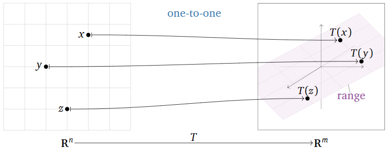
$Grid with three parallelograms, each originating from a point labeled X. Lines connect X to each parallelogram at labeled vertices F1(x), F2(x), and F3(x). Background reads OD + CK sum.$

Figure $\PageIndex{1}$

Here are some equivalent ways of saying that $T$ is not one-to-one:

There exists some vector $b$ in $\mathbb{R}^m $ such that the equation $T(x)=b$ has more than one solution $x$ in $\mathbb{R}^n $.
There are two different inputs of $T$ with the same output.
There exist vectors $u,v$ such that $u\neq v$ but $T(u)=T(v)$.

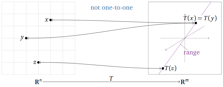
$Diagram illustrating a linear transformation from sets $X$ to $Y$. Points in $X$ map to corresponding points in $Y$. Contains lines, grids, and labeled vectors within a transformation box.$

Figure $\PageIndex{2}$

Example $\PageIndex{1}$: Functions of one variable

The function $\sin\colon \mathbb{R} \to\mathbb{R} $ is not one-to-one. Indeed, $\sin(0) = \sin(\pi) = 0\text{,}$ so the inputs $0$ and $\pi$ have the same output $0$. In fact, the equation $\sin(x) = 0$ has infinitely many solutions $\ldots,-2\pi,-\pi,0,\pi,2\pi,\ldots$.

The function $\exp\colon \mathbb{R} \to\mathbb{R} $ defined by $\exp(x) = e^x$ is one-to-one. Indeed, if $T(x) = T(y)\text{,}$ then $e^x = e^y\text{,}$ so $\ln(e^x) = \ln(e^y)\text{,}$ and hence $x = y$. The equation $T(x) = C$ has one solution $x = \ln(C)$ if $C > 0\text{,}$ and it has zero solutions if $C\leq 0$.

The function $f\colon \mathbb{R} \to\mathbb{R} $ defined by $f(x)=x^3$ is one-to-one. Indeed, if $f(x) = f(y)$ then $x^3 = y^3\text{;}$ taking cube roots gives $x = y$. In other words, the only solution of $f(x) = C$ is $x=\sqrt[3]C$.

The function $f\colon \mathbb{R} \to\mathbb{R} $ defined by $f(x)=x^3-x$ is not one-to-one. Indeed, $f(0) = f(1) = f(-1) = 0\text{,}$ so the inputs $0,1,-1$ all have the same output $0$. The solutions of the equation $x^3 - x = 0$ are exactly the roots of $f(x) = x(x-1)(x+1)\text{,}$ and this equation has three roots.

The function $f\colon \mathbb{R} \to\mathbb{R} $ defined by $f(x)=x^2$ is not one-to-one. Indeed, $f(1) = 1 = f(-1)\text{,}$ so the inputs $1$ and $-1$ have the same outputs. The function $g\colon \mathbb{R} \to\mathbb{R} $ defined by $g(x)=|x|$ is not one-to-one for the same reason.

Example $\PageIndex{2}$: A real-word transformation: robotics

Suppose you are building a robot arm with three joints that can move its hand around a plane, as in Example 3.1.11 in Section 3.1.

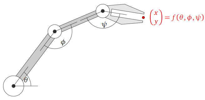
$Diagram of a robotic arm with three segments and rotational joints. The end effector is marked in red, labeled as $f(\theta, \phi, \psi)$. Angles $\theta$, $\phi$, and $\psi$ are indicated.$

Figure $\PageIndex{3}$

Define a transformation $f\colon\mathbb{R}^3 \to\mathbb{R}^2 $ as follows: $f(\theta,\phi,\psi)$ is the $(x,y)$ position of the hand when the joints are rotated by angles $\theta, \phi, \psi\text{,}$ respectively. Asking whether $f$ is one-to-one is the same as asking whether there is more than one way to move the arm in order to reach your coffee cup. (There is.)

Theorem $\PageIndex{1}$: One-to-One Matrix Transformations

Let $A$ be an $m\times n$ matrix, and let $T(x)=Ax$ be the associated matrix transformation. The following statements are equivalent:

$T$ is one-to-one.
For every $b$ in $\mathbb{R}^m \text{,}$ the equation $T(x)=b$ has at most one solution.
For every $b$ in $\mathbb{R}^m \text{,}$ the equation $Ax=b$ has a unique solution or is inconsistent.
$Ax=0$ has only the trivial solution.
The columns of $A$ are linearly independent.
$A$ has a pivot in every column.
The range of $T$ has dimension $n$.

Proof: Statements 1, 2, and 3 are translations of each other. The equivalence of 3 and 4 follows from key observation 2.4.3 in Section 2.4: if $Ax=0$ has only one solution, then $Ax=b$ has only one solution as well, or it is inconsistent. The equivalence of 4, 5, and 6 is a consequence of Recipe: Checking Linear Independence in Section 2.5, and the equivalence of 6 and 7 follows from the fact that the rank of a matrix is equal to the number of columns with pivots.

Recall that equivalent means that, for a given matrix, either all of the statements are true simultaneously, or they are all false.

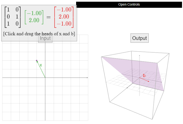
Example $\PageIndex{3}$: A matrix transformation that is one-to-one

Let $A$ be the matrix

\[A=\left(\begin{array}{cc}1&0\\0&1\\1&0\end{array}\right),\nonumber\]

and define $T\colon\mathbb{R}^2 \to\mathbb{R}^3 $ by $T(x) = Ax$. Is $T$ one-to-one?

Solution

The reduced row echelon form of $A$ is

\[\left(\begin{array}{cc}1&0\\0&1\\0&0\end{array}\right).\nonumber\]

Hence $A$ has a pivot in every column, so $T$ is one-to-one.

$3D linear transformation illustration. Left: Input vector and transformation matrix. Right: Output vector and shaded plane showing transformation effect in 3D space.$

Figure $\PageIndex{4}$: A picture of the matrix transformation $T$. As you drag the input vector on the left side, you see that different input vectors yield different output vectors on the right side.

Example $\PageIndex{4}$: A matrix transformation that is not one-to-one

Let

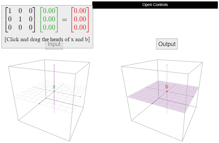
\[A=\left(\begin{array}{ccc}1&0&0\\0&1&0\\0&0&0\end{array}\right),\nonumber\]

and define $T\colon\mathbb{R}^3 \to\mathbb{R}^3 $ by $T(x) = Ax$. Is $T$ one-to-one? If not, find two different vectors $u,v$ such that $T(u)=T(v)$.

Solution

The matrix $A$ is already in reduced row echelon form. It does not have a pivot in every column, so $T$ is not one-to-one. Therefore, we know from the Theorem $\PageIndex{1}$ that $Ax=0$ has nontrivial solutions. If $v$ is a nontrivial (i.e., nonzero) solution of $Av = 0\text{,}$ then $T(v) = Av = 0 = A0 = T(0)\text{,}$ so $0$ and $v$ are different vectors with the same output. For instance,

\[T\left(\begin{array}{c}0\\0\\1\end{array}\right)=\left(\begin{array}{ccc}1&0&0\\0&1&0\\0&0&0\end{array}\right)\:\left(\begin{array}{c}0\\0\\1\end{array}\right)=0=T\left(\begin{array}{c}0\\0\\0\end{array}\right).\nonumber\]

Geometrically, $T$ is projection onto the $xy$-plane. Any two vectors that lie on the same vertical line will have the same projection. For $b$ on the $xy$-plane, the solution set of $T(x) = b$ is the entire vertical line containing $b$. In particular, $T(x) = b$ has infinitely many solutions.

$A 3D graph comparing inputs and outputs of a matrix operation, showing a transformation with sliders to adjust coefficients. Input on the left, output on the right.$

Figure $\PageIndex{5}$: A picture of the matrix transformation $T$. The transformation $T$ projects a vector onto the $xy$-plane. The violet line is the solution set of $T(x)=0$. If you drag $x$ along the violet line, the output $T(x) = Ax$ does not change. This demonstrates that $T(x)=0$ has more than one solution, so $T$ is not one-to-one.

Example $\PageIndex{5}$: A matrix transformation that is not one-to-one

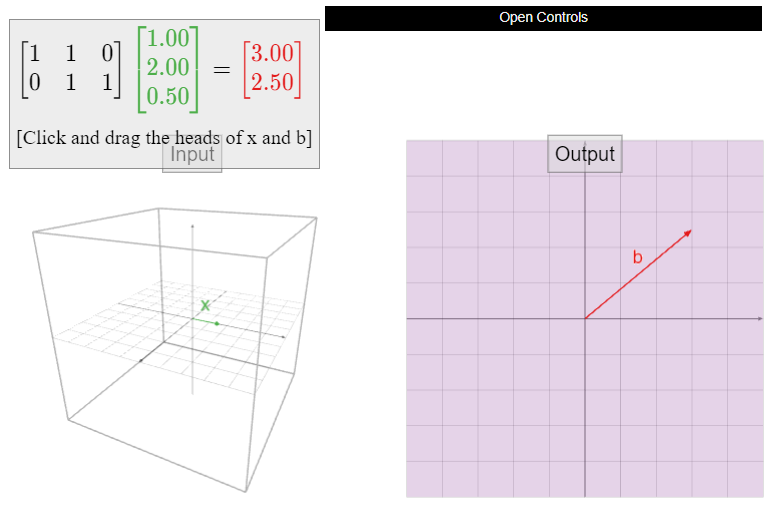
Let $A$ be the matrix

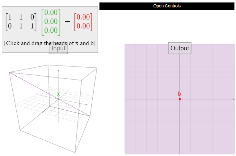
\[A=\left(\begin{array}{ccc}1&1&0\\0&1&1\end{array}\right),\nonumber\]

and define $T\colon\mathbb{R}^3 \to\mathbb{R}^2 $ by $T(x) = Ax$. Is $T$ one-to-one? If not, find two different vectors $u,v$ such that $T(u)=T(v)$.

Solution

The reduced row echelon form of $A$ is

\[\left(\begin{array}{ccc}1&0&-1\\0&1&1\end{array}\right).\nonumber\]

There is not a pivot in every column, so $T$ is not one-to-one. Therefore, we know from Theorem $\PageIndex{1}$ that $Ax=0$ has nontrivial solutions. If $v$ is a nontrivial (i.e., nonzero) solution of $Av = 0\text{,}$ then $T(v) = Av = 0 = A0 = T(0)\text{,}$ so $0$ and $v$ are different vectors with the same output. In order to find a nontrivial solution, we find the parametric form of the solutions of $Ax=0$ using the reduced matrix above:

\[\left\{\begin{array}{rrrrrrr}x &{}&{}& -& z &=& 0\\ {}&{}& y& + &z &=& 0\end{array}\right.\quad\implies\quad\left\{\begin{array}{rrr}x&=&z \\ y&=&-z\end{array}\right.\nonumber\]

The free variable is $z$. Taking $z=1$ gives the nontrivial solution

\[T\left(\begin{array}{c}1\\-1\\1\end{array}\right)=\left(\begin{array}{ccc}1&1&0\\0&1&1\end{array}\right)\:\left(\begin{array}{c}1\\-1\\1\end{array}\right)=0=T\left(\begin{array}{c}0\\0\\0\end{array}\right).\nonumber\]

$3D vector matrix on the left transforms to red and green point matrix. Right displays a 2D graph with Output text and a red point.$

Figure $\PageIndex{6}$: A picture of the matrix transformation $T$. The violet line is the null space of $A\text{,}$ i.e., solution set of $T(x)=0$. If you drag $x$ along the violet line, the output $T(x) = Ax$ does not change. This demonstrates that $T(x)=0$ has more than one solution, so $T$ is not one-to-one.

Example $\PageIndex{6}$: A matrix transformation that is not one-to-one

Let

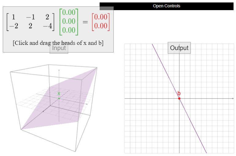
\[A=\left(\begin{array}{ccc}1&-1&2\\-2&2&-4\end{array}\right),\nonumber\]

and define $T\colon\mathbb{R}^3 \to\mathbb{R}^2 $ by $T(x) = Ax$. Is $T$ one-to-one? If not, find two different vectors $u,v$ such that $T(u)=T(v)$.

Solution

The reduced row echelon form of $A$ is

\[\left(\begin{array}{ccc}1&-1&2\\0&0&0\end{array}\right).\nonumber\]

\[ x - y + 2z = 0 \quad\implies\quad x = y - 2z. \nonumber \]

The free variables are $y$ and $z$. Taking $y=1$ and $z=0$ gives the nontrivial solution

\[T\left(\begin{array}{c}1\\1\\0\end{array}\right)=\left(\begin{array}{ccc}1&-1&2\\-2&2&-4\end{array}\right)\:\left(\begin{array}{c}1\\1\\0\end{array}\right)=0=T\left(\begin{array}{c}0\\0\\0\end{array}\right).\nonumber\]

$A 3D graph on the left depicts a purple plane and a black intersecting line, with input box vectors. The right contains an Output section with a red point on a grid, intersecting a diagonal line.$

Figure $\PageIndex{7}$: A picture of the matrix transformation $T$. The violet plane is the solution set of $T(x)=0$. If you drag $x$ along the violet plane, the output $T(x) = Ax$ does not change. This demonstrates that $T(x)=0$ has more than one solution, so $T$ is not one-to-one.

The previous three examples can be summarized as follows. Suppose that $T(x)=Ax$ is a matrix transformation that is not one-to-one. By Theorem $\PageIndex{1}$, there is a nontrivial solution of $Ax=0$. This means that the null space of $A$ is not the zero space. All of the vectors in the null space are solutions to $T(x)=0$. If you compute a nonzero vector $v$ in the null space (by row reducing and finding the parametric form of the solution set of $Ax=0\text{,}$ for instance), then $v$ and $0$ both have the same output: $T(v) = Av = 0 = T(0).$

Note $\PageIndex{1}$: Wide matrices do not have one-to-one transformations

If $T\colon\mathbb{R}^n \to\mathbb{R}^m $ is a one-to-one matrix transformation, what can we say about the relative sizes of $n$ and $m\text{?}$

The matrix associated to $T$ has $n$ columns and $m$ rows. Each row and each column can only contain one pivot, so in order for $A$ to have a pivot in every column, it must have at least as many rows as columns: $n\leq m$.

This says that, for instance, $\mathbb{R}^3 $ is “too big” to admit a one-to-one linear transformation into $\mathbb{R}^2 $.

Note that there exist tall matrices that are not one-to-one: for example,

\[\left(\begin{array}{ccc}1&0&0\\0&1&0\\0&0&0\\0&0&0\end{array}\right)\nonumber\]

does not have a pivot in every column.

Onto Transformations

Definition $\PageIndex{2}$: Onto transformations

A transformation $T\colon\mathbb{R}^n \to\mathbb{R}^m $ is onto if, for every vector $b$ in $\mathbb{R}^m \text{,}$ the equation $T(x)=b$ has at least one solution $x$ in $\mathbb{R}^n $.

Remark

Another word for onto is surjective.

Here are some equivalent ways of saying that $T$ is onto:

The range of $T$ is equal to the codomain of $T$.
Every vector in the codomain is the output of some input vector.

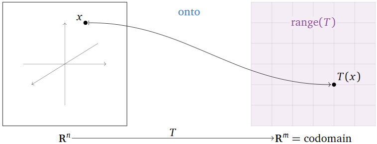
$Diagram illustrating a mathematical transformation $ T $. A point $ x $ transforms to $ T(x) $, with domains and ranges labeled. Arrow shows movement from input to output space.$

Figure $\PageIndex{8}$

Here are some equivalent ways of saying that $T$ is not onto:

The range of $T$ is smaller than the codomain of $T$.
There exists a vector $b$ in $\mathbb{R}^m $ such that the equation $T(x)=b$ does not have a solution.
There is a vector in the codomain that is not the output of any input vector.

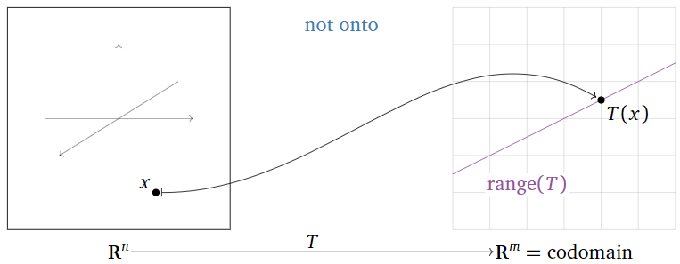
$Diagram showing a transformation map from set X (left box) to its image in set Y (right box). X is R^n, Y is R^m coordinates. A dashed arrow indicates mapping T(x) from X to range(T).$

Figure $\PageIndex{9}$

Example $\PageIndex{7}$: Functions of one variable

The function $\sin\colon \mathbb{R} \to\mathbb{R} $ is not onto. Indeed, taking $b=2\text{,}$ the equation $\sin(x)=2$ has no solution. The range of $\sin$ is the closed interval $[-1,1]\text{,}$ which is smaller than the codomain $\mathbb{R}$.

The function $\exp\colon \mathbb{R} \to\mathbb{R} $ defined by $\exp(x) = e^x$ is not onto. Indeed, taking $b=-1\text{,}$ the equation $\exp(x) = e^x = -1$ has no solution. The range of $\exp$ is the set $(0,\infty)$ of all positive real numbers.

The function $f\colon \mathbb{R} \to\mathbb{R} $ defined by $f(x)=x^3$ is onto. Indeed, the equation $f(x) = x^3 = b$ always has the solution $x = \sqrt[3]b$.

The function $f\colon \mathbb{R} \to\mathbb{R} $ defined by $f(x)=x^3-x$ is onto. Indeed, the solutions of the equation $f(x) = x^3 - x = b$ are the roots of the polynomial $x^3 - x - b\text{;}$ as this is a cubic polynomial, it has at least one real root.

Example $\PageIndex{8}$: A real-word transformation: robotics

The robot arm transformation of Example $\PageIndex{2}$ is not onto. The robot cannot reach objects that are very far away.

Theorem $\PageIndex{2}$: Onto Matrix Transformations

Let $A$ be an $m\times n$ matrix, and let $T(x)=Ax$ be the associated matrix transformation. The following statements are equivalent:

$T$ is onto.
$T(x)=b$ has at least one solution for every $b$ in $\mathbb{R}^m $.
$Ax=b$ is consistent for every $b$ in $\mathbb{R}^m $.
The columns of $A$ span $\mathbb{R}^m $.
$A$ has a pivot in every row.
The range of $T$ has dimension $m$.

Proof: Statements 1, 2, and 3 are translations of each other. The equivalence of 3, 4, 5, and 6 follows from Theorem 2.3.1 in Section 2.3.

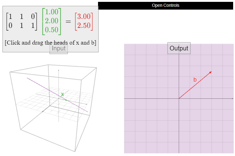
Example $\PageIndex{9}$: A matrix transformation that is onto

Let $A$ be the matrix

\[A=\left(\begin{array}{ccc}1&1&0\\0&1&1\end{array}\right),\nonumber\]

and define $T\colon\mathbb{R}^3 \to\mathbb{R}^2 $ by $T(x) = Ax$. Is $T$ onto?

Solution

The reduced row echelon form of $A$ is

\[\left(\begin{array}{ccc}1&0&-1\\0&1&1\end{array}\right).\nonumber\]

Hence $A$ has a pivot in every row, so $T$ is onto.

$Matrix transformation tool showing a 2x2 matrix transforming a vector from input to output. The vector changes in both direction and magnitude as shown on a 3D graph and a 2D output grid.$

Figure $\PageIndex{10}$: A picture of the matrix transformation $T$. Every vector on the right side is the output of $T$ for a suitable input. If you drag $b\text{,}$ the demo will find an input vector $x$ with output $b$.

Example $\PageIndex{10}$: A matrix transformation that is not onto

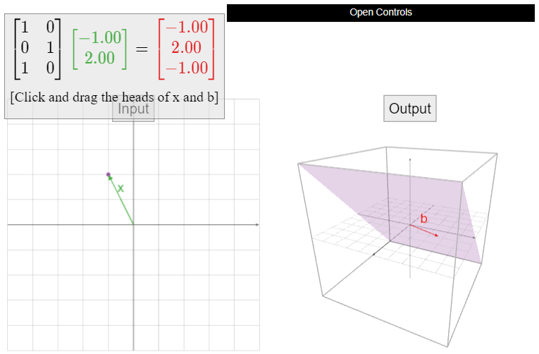
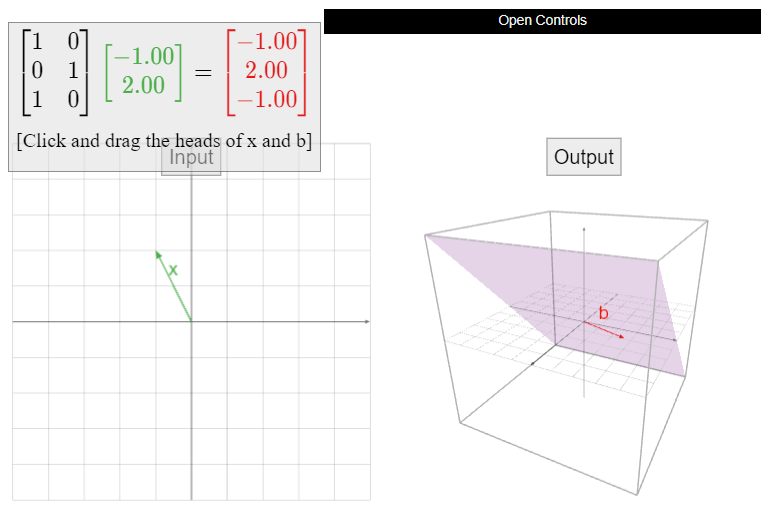
Let $A$ be the matrix

\[A=\left(\begin{array}{cc}1&0\\0&1\\1&0\end{array}\right),\nonumber\]

and define $T\colon\mathbb{R}^2 \to\mathbb{R}^3 $ by $T(x) = Ax$. Is $T$ onto? If not, find a vector $b$ in $\mathbb{R}^3 $ such that $T(x)=b$ has no solution.

Solution

The reduced row echelon form of $A$ is

\[\left(\begin{array}{cc}1&0\\0&1\\0&0\end{array}\right).\nonumber\]

Hence $A$ does not have a pivot in every row, so $T$ is not onto. In fact, since

\[T\left(\begin{array}{c}x\\y\end{array}\right)=\left(\begin{array}{cc}1&0\\0&1\\1&0\end{array}\right)\:\left(\begin{array}{c}x\\y\end{array}\right)=\left(\begin{array}{c}x\\y\\x\end{array}\right),\nonumber\]

we see that for every output vector of $T\text{,}$ the third entry is equal to the first. Therefore,

\[ b=(1,2,3) \nonumber \]

is not in the range of $T$.

$Two matrices and a 3D graph. The left matrix has sliders; the right matrix shows values. Below is a 2D grid with a green vector. Right displays a 3D plot with a red vector, labeled Output.$

Figure $\PageIndex{11}$: A picture of the matrix transformation $T$. The range of $T$ is the violet plane on the right; this is smaller than the codomain $\mathbb{R}^3 $. If you drag $b$ off of the violet plane, then the equation $Ax=b$ becomes inconsistent; this means $T(x)=b$ has no solution.

Example $\PageIndex{11}$: A matrix transformation that is not onto

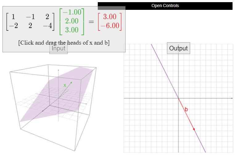
Let

\[A=\left(\begin{array}{ccc}1&-1&2\\-2&2&4\end{array}\right),\nonumber\]

and define $T\colon\mathbb{R}^3 \to\mathbb{R}^2 $ by $T(x) = Ax$. Is $T$ onto? If not, find a vector $b$ in $\mathbb{R}^2 $ such that $T(x)=b$ has no solution.

Solution

The reduced row echelon form of $A$ is

\[\left(\begin{array}{ccc}1&-1&2\\0&0&0\end{array}\right).\nonumber\]

There is not a pivot in every row, so $T$ is not onto. The range of $T$ is the column space of $A\text{,}$ which is equal to

\[\text{Span}\left\{\left(\begin{array}{c}1\\-2\end{array}\right),\:\left(\begin{array}{c}-1\\2\end{array}\right),\:\left(\begin{array}{c}2\\-4\end{array}\right)\right\}=\text{Span}\left\{\left(\begin{array}{c}1\\-2\end{array}\right)\right\},\nonumber\]

since all three columns of $A$ are collinear. Therefore, any vector not on the line through $1\choose-2$ is not in the range of $T$. For instance, if $b={1\choose 1}$ then $T(x)=b$ has no solution.

$Matrix transformation example: a 2x2 matrix transforming a 3D vector, shown in a graph. The matrix alters the vector from [3.00, 3.00] to [3.00, -6.00].$

Figure $\PageIndex{12}$: A picture of the matrix transformation $T$. The range of $T$ is the violet line on the right; this is smaller than the codomain $\mathbb{R}^2 $. If you drag $b$ off of the violet line, then the equation $Ax=b$ becomes inconsistent; this means $T(x)=b$ has no solution.

The previous two examples illustrate the following observation. Suppose that $T(x)=Ax$ is a matrix transformation that is not onto. This means that $\text{range}(T) = \text{Col}(A)$ is a subspace of $\mathbb{R}^m $ of dimension less than $m\text{:}$ perhaps it is a line in the plane, or a line in $3$-space, or a plane in $3$-space, etc. Whatever the case, the range of $T$ is very small compared to the codomain. To find a vector not in the range of $T\text{,}$ choose a random nonzero vector $b$ in $\mathbb{R}^m \text{;}$ you have to be extremely unlucky to choose a vector that is in the range of $T$. Of course, to check whether a given vector $b$ is in the range of $T\text{,}$ you have to solve the matrix equation $Ax=b$ to see whether it is consistent.

Note $\PageIndex{2}$: Tall matrices do not have onto transformations

If $T\colon\mathbb{R}^n \to\mathbb{R}^m $ is an onto matrix transformation, what can we say about the relative sizes of $n$ and $m\text{?}$

The matrix associated to $T$ has $n$ columns and $m$ rows. Each row and each column can only contain one pivot, so in order for $A$ to have a pivot in every row, it must have at least as many columns as rows: $m\leq n$.

This says that, for instance, $\mathbb{R}^2 $ is “too small” to admit an onto linear transformation to $\mathbb{R}^3 $.

Note that there exist wide matrices that are not onto: for example,

\[\left(\begin{array}{ccc}1&-1&2\\-2&2&-4\end{array}\right)\nonumber\]

does not have a pivot in every row.

Comparison

The above expositions of one-to-one and onto transformations were written to mirror each other. However, “one-to-one” and “onto” are complementary notions: neither one implies the other. Below we have provided a chart for comparing the two. In the chart, $A$ is an $m\times n$ matrix, and $T\colon\mathbb{R}^n \to\mathbb{R}^m $ is the matrix transformation $T(x)=Ax$.

Table $\PageIndex{1}$

$T$ is one-to-one	$T$ is onto
$T(x)=b$ has at most one solution for every $b$.	$T(x)=b$ has at least one solution for every $b$.
The columns of $A$ are linearly independent.	The columns of $A$ span $\mathbb{R}^m$.
$A$ has a pivot column in every column.	$A$ has a pivot in every row.
The range of $T$ has dimension $n$.	The range of $T$ has dimension $m$.

Example $\PageIndex{12}$: Functions of one variable

The function $\sin\colon \mathbb{R} \to\mathbb{R} $ is neither one-to-one nor onto.

The function $\exp\colon \mathbb{R} \to\mathbb{R} $ defined by $\exp(x) = e^x$ is one-to-one but not onto.

The function $f\colon \mathbb{R} \to\mathbb{R} $ defined by $f(x)=x^3$ is one-to-one and onto.

The function $f\colon \mathbb{R} \to\mathbb{R} $ defined by $f(x)=x^3-x$ is onto but not one-to-one.

Example $\PageIndex{13}$: A matrix transformation that is neither one-to-one nor onto

Let

\[A=\left(\begin{array}{ccc}1&-1&2\\-2&2&-4\end{array}\right),\nonumber\]

and define $T\colon\mathbb{R}^3 \to\mathbb{R}^2 $ by $T(x) = Ax$. This transformation is neither one-to-one nor onto, as we saw in Example $\PageIndex{6}$ and Example $\PageIndex{11}$.

$Matrix equation solving with two 3D planes intersecting at a line, shown on the left. On the right, a graph with Output labeled, displaying the intersection point on the vertical axis.$

Figure $\PageIndex{13}$: A picture of the matrix transformation $T$. The violet plane is the solution set of $T(x)=0$. If you drag $x$ along the violet plane, the output $T(x) = Ax$ does not change. This demonstrates that $T(x)=0$ has more than one solution, so $T$ is not one-to-one. The range of $T$ is the violet line on the right; this is smaller than the codomain $\mathbb{R}^2 $. If you drag $b$ off of the violet line, then the equation $Ax=b$ becomes inconsistent; this means $T(x)=b$ has no solution.

Example $\PageIndex{14}$: A matrix transformation that is one-to-one but not onto

Let $A$ be the matrix

\[A=\left(\begin{array}{cc}1&0\\0&1\\1&0\end{array}\right),\nonumber\]

and define $T\colon\mathbb{R}^2 \to\mathbb{R}^3 $ by $T(x) = Ax$. This transformation is one-to-one but not onto, as we saw in this Example $\PageIndex{3}$ and this Example $\PageIndex{10}$.

$A graphical representation of a 2D transformation matrix acting on a vector, displayed in an input-output format. The input shows a vector in a grid, and the output showcases the transformed vector in 3D space.$

Figure $\PageIndex{14}$: A picture of the matrix transformation $T$. The range of $T$ is the violet plane on the right; this is smaller than the codomain $\mathbb{R}^3 $. If you drag $b$ off of the violet plane, then the equation $Ax=b$ becomes inconsistent; this means $T(x)=b$ has no solution. However, for $b$ lying on the violet plane, there is a unique vector $x$ such that $T(x)=b$.

Example $\PageIndex{15}$: A matrix transformation that is onto but not one-to-one

Let $A$ be the matrix

\[A=\left(\begin{array}{ccc}1&1&0\\0&1&1\end{array}\right),\nonumber\]

and define $T\colon\mathbb{R}^3 \to\mathbb{R}^2 $ by $T(x) = Ax$. This transformation is onto but not one-to-one, as we saw in Example $\PageIndex{9}$.

$Matrix transformation shown on the left with a 3D graph and corresponding 2D output graph on the right. Arrow labeled b projects from the transformation onto a purple grid.$

Figure $\PageIndex{15}$: A picture of the matrix transformation $T$. Every vector on the right side is the output of $T$ for a suitable input. If you drag $b\text{,}$ the demo will find an input vector $x$ with output $b$. The violet line is the null space of $A\text{,}$ i.e., solution set of $T(x)=0$. If you drag $x$ along the violet line, the output $T(x) = Ax$ does not change. This demonstrates that $T(x)=0$ has more than one solution, so $T$ is not one-to-one.

Example $\PageIndex{16}$: Matrix transformations that are both one-to-one and onto

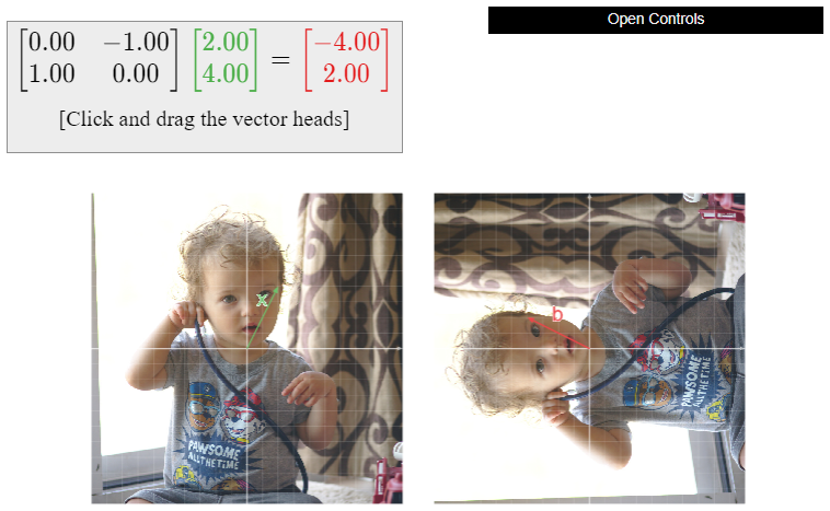
In Subsection Matrices as Functions in Section 3.1, we discussed the transformations defined by several $2\times 2$ matrices, namely:

\begin{align*} \text{Reflection:} &\qquad A=\left(\begin{array}{cc}-1&0\\0&1\end{array}\right) \\ \text{Dilation:} &\qquad A=\left(\begin{array}{cc}1.5&0\\0&1.5\end{array}\right) \\ \text{Identity:} &\qquad A=\left(\begin{array}{cc}1&0\\0&1\end{array}\right) \\ \text{Rotation:} &\qquad A=\left(\begin{array}{cc}0&-1\\1&0\end{array}\right) \\ \text{Shear:} &\qquad A=\left(\begin{array}{cc}1&1\\0&1\end{array}\right). \end{align*}

In each case, the associated matrix transformation $T(x)=Ax$ is both one-to-one and onto. A $2\times 2$ matrix $A$ has a pivot in every row if and only if it has a pivot in every column (if and only if it has two pivots), so in this case, the transformation $T$ is one-to-one if and only if it is onto. One can see geometrically that they are onto (what is the input for a given output?), or that they are one-to-one using the fact that the columns of $A$ are not collinear.

$A split image showing a matrix transformation applied to a photo. Left: matrix values and vectors. Right: child seen through a window, one image unaltered, the other skewed by the transformation.$

Figure $\PageIndex{16}$: Counterclockwise rotation by $90^\circ$ is a matrix transformation. This transformation is onto (if $b$ is a vector in $\mathbb{R}^2 \text{,}$ then it is the output vector for the input vector which is $b$ rotated clockwise by $90^\circ$), and it is one-to-one (different vectors rotate to different vectors).

Note $\PageIndex{3}$: One-to-one is the same as onto for square matrices

We observed in the previous Example $\PageIndex{16}$ that a square matrix has a pivot in every row if and only if it has a pivot in every column. Therefore, a matrix transformation $T$ from $\mathbb{R}^n $ to itself is one-to-one if and only if it is onto: in this case, the two notions are equivalent.

Conversely, by Note $\PageIndex{1}$ and Note $\PageIndex{2}$, if a matrix transformation $T\colon\mathbb{R}^m \to\mathbb{R}^n $ is both one-to-one and onto, then $m=n$.

Note that in general, a transformation $T$ is both one-to-one and onto if and only if $T(x)=b$ has exactly one solution for all $b$ in $\mathbb{R}^m $.

\(T\) is one-to-one	\(T\) is onto
\(T(x)=b\) has at most one solution for every \(b\).	\(T(x)=b\) has at least one solution for every \(b\).
The columns of \(A\) are linearly independent.	The columns of \(A\) span \(\mathbb{R}^m\).
\(A\) has a pivot column in every column.	\(A\) has a pivot in every row.
The range of \(T\) has dimension \(n\).	The range of \(T\) has dimension \(m\).

Search

Text Color

Text Size

Margin Size

Font Type

Definition \(\PageIndex{1}\): One-to-one transformations

Remark

Example \(\PageIndex{1}\): Functions of one variable

Example \(\PageIndex{2}\): A real-word transformation: robotics

Theorem \(\PageIndex{1}\): One-to-One Matrix Transformations

Example \(\PageIndex{3}\): A matrix transformation that is one-to-one

Solution

Example \(\PageIndex{4}\): A matrix transformation that is not one-to-one

Solution

Example \(\PageIndex{5}\): A matrix transformation that is not one-to-one

Solution

Example \(\PageIndex{6}\): A matrix transformation that is not one-to-one

Solution

Note \(\PageIndex{1}\): Wide matrices do not have one-to-one transformations

Definition \(\PageIndex{2}\): Onto transformations

Remark

Example \(\PageIndex{7}\): Functions of one variable

Example \(\PageIndex{8}\): A real-word transformation: robotics

Theorem \(\PageIndex{2}\): Onto Matrix Transformations

Example \(\PageIndex{9}\): A matrix transformation that is onto

Solution

Example \(\PageIndex{10}\): A matrix transformation that is not onto

Solution

Example \(\PageIndex{11}\): A matrix transformation that is not onto

Solution

Note \(\PageIndex{2}\): Tall matrices do not have onto transformations

Example \(\PageIndex{12}\): Functions of one variable

Example \(\PageIndex{13}\): A matrix transformation that is neither one-to-one nor onto

Example \(\PageIndex{14}\): A matrix transformation that is one-to-one but not onto

Example \(\PageIndex{15}\): A matrix transformation that is onto but not one-to-one

Example \(\PageIndex{16}\): Matrix transformations that are both one-to-one and onto

Note \(\PageIndex{3}\): One-to-one is the same as onto for square matrices