5.1: Eigenvalues and Eigenvectors

\(\usepackage{macros} \newcommand{\lt}{<} \newcommand{\gt}{>} \newcommand{\amp}{&} \)

Learning Objectives

1. Learn the definition of eigenvector and eigenvalue.
2. Learn to find eigenvectors and eigenvalues geometrically.
3. Learn to decide if a number is an eigenvalue of a matrix, and if so, how to find an associated eigenvector.
4. Recipe: find a basis for the \(\lambda\)-eigenspace.
5. Pictures: whether or not a vector is an eigenvector, eigenvectors of standard matrix transformations.
6. Theorem: the expanded invertible matrix theorem.
7. Vocabulary word: eigenspace.
8. Essential vocabulary words: eigenvector, eigenvalue.

In this section, we define eigenvalues and eigenvectors. These form the most important facet of the structure theory of square matrices. As such, eigenvalues and eigenvectors tend to play a key role in the real-life applications of linear algebra.

Eigenvalues and Eigenvectors

Here is the most important definition in this text.

Definition \(\PageIndex{1}\): Eigenvector and Eigenvalue

Let \(A\) be an \(n\times n\) matrix.

1. An eigenvector of \(A\) is a nonzero vector \(v\) in \(\mathbb{R}^n \) such that \(Av=\lambda v\text{,}\) for some scalar \(\lambda\).
2. An eigenvalue of \(A\) is a scalar \(\lambda\) such that the equation \(Av=\lambda v\) has a nontrivial solution.

If \(Av = \lambda v\) for \(v\neq 0\text{,}\) we say that \(\lambda\) is the eigenvalue for \(v\text{,}\) and that \(v\) is an eigenvector for \(\lambda\).

The German prefix “eigen” roughly translates to “self” or “own”. An eigenvector of \(A\) is a vector that is taken to a multiple of itself by the matrix transformation \(T(x)=Ax\text{,}\) which perhaps explains the terminology. On the other hand, “eigen” is often translated as “characteristic”; we may think of an eigenvector as describing an intrinsic, or characteristic, property of \(A\).

Note \(\PageIndex{1}\)

Eigenvalues and eigenvectors are only for square matrices.

Note \(\PageIndex{2}\)

Eigenvectors are by definition nonzero. Eigenvalues may be equal to zero.

We do not consider the zero vector to be an eigenvector: since \(A0 = 0 = \lambda 0\) for every scalar \(\lambda\text{,}\) the associated eigenvalue would be undefined.

If someone hands you a matrix \(A\) and a vector \(v\text{,}\) it is easy to check if \(v\) is an eigenvector of \(A\text{:}\) simply multiply \(v\) by \(A\) and see if \(Av\) is a scalar multiple of \(v\). On the other hand, given just the matrix \(A\text{,}\) it is not obvious at all how to find the eigenvectors. We will learn how to do this in Section 5.2.

Example \(\PageIndex{1}\): Verifying eigenvectors

Consider the matrix

\[ A = \left(\begin{array}{cc}2&2\\-4&8\end{array}\right)\qquad\text{and vectors}\qquad v = \left(\begin{array}{c}1\\1\end{array}\right) \qquad w = \left(\begin{array}{c}2\\1\end{array}\right). \nonumber \]

Which are eigenvectors? What are their eigenvalues?

Solution

We have

\[ Av = \left(\begin{array}{cc}2&2\\-4&8\end{array}\right)\left(\begin{array}{c}1\\1\end{array}\right)=\left(\begin{array}{c}4\\4\end{array}\right) = 4v. \nonumber \]

Hence, \(v\) is an eigenvector of \(A\text{,}\) with eigenvalue \(\lambda = 4\). On the other hand,

\[ Aw = \left(\begin{array}{cc}2&2\\-4&8\end{array}\right)\left(\begin{array}{c}2\\1\end{array}\right)=\left(\begin{array}{c}6\\0\end{array}\right). \nonumber \]

which is not a scalar multiple of \(w\). Hence, \(w\) is not an eigenvector of \(A\).

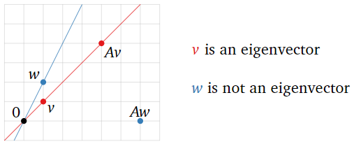
Figure \(\PageIndex{1}\)

Example \(\PageIndex{2}\): Verifying eigenvectors

Consider the matrix

\[ A = \left(\begin{array}{ccc}0&6&8\\ \frac{1}{2}&0&0\\0&\frac{1}{2}&0\end{array}\right)\qquad\text{and vectors}\qquad v = \left(\begin{array}{c}16\\4\\1\end{array}\right) \qquad w = \left(\begin{array}{c}2\\2\\2\end{array}\right). \nonumber \]

Which are eigenvectors? What are their eigenvalues?

Solution

We have

\[ Av = \left(\begin{array}{ccc}0&6&8\\ \frac{1}{2}&0&0\\0&\frac{1}{2}&0\end{array}\right) \left(\begin{array}{c}16\\4\\1\end{array}\right) = \left(\begin{array}{c}32\\8\\2\end{array}\right) = 2v. \nonumber \]

Hence, \(v\) is an eigenvector of \(A\text{,}\) with eigenvalue \(\lambda = 2\). On the other hand,

\[ Aw = \left(\begin{array}{ccc}0&6&8\\ \frac{1}{2}&0&0\\0&\frac{1}{2}&0\end{array}\right)\left(\begin{array}{c}2\\2\\2\end{array}\right) = \left(\begin{array}{c}28\\1\\1\end{array}\right), \nonumber \]

which is not a scalar multiple of \(w\). Hence, \(w\) is not an eigenvector of \(A\).

Example \(\PageIndex{3}\): An eigenvector with eigenvalue \(0\)

Let

\[ A = \left(\begin{array}{cc}1&3\\2&6\end{array}\right) \qquad v =\left(\begin{array}{c}-3\\1\end{array}\right). \nonumber \]

Is \(v\) an eigenvector of \(A\text{?}\) If so, what is its eigenvalue?

Solution

The product is

\[ Av = \left(\begin{array}{cc}1&3\\2&6\end{array}\right)\left(\begin{array}{c}-3\\1\end{array}\right) = \left(\begin{array}{c}0\\0\end{array}\right) = 0v. \nonumber \]

Hence, \(v\) is an eigenvector with eigenvalue zero.

As noted above, an eigenvalue is allowed to be zero, but an eigenvector is not.

To say that \(Av=\lambda v\) means that \(Av\) and \(\lambda v\) are collinear with the origin. So, an eigenvector of \(A\) is a nonzero vector \(v\) such that \(Av\) and \(v\) lie on the same line through the origin. In this case, \(Av\) is a scalar multiple of \(v\text{;}\) the eigenvalue is the scaling factor.

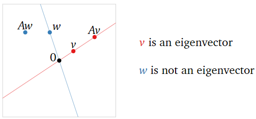
Figure \(\PageIndex{2}\)

For matrices that arise as the standard matrix of a linear transformation, it is often best to draw a picture, then find the eigenvectors and eigenvalues geometrically by studying which vectors are not moved off of their line. For a transformation that is defined geometrically, it is not necessary even to compute its matrix to find the eigenvectors and eigenvalues.

Example \(\PageIndex{4}\): Reflection

Here is an example of this. Let \(T\colon\mathbb{R}^2\to\mathbb{R}^2\) be the linear transformation that reflects over the line \(L\) defined by \(y=-x\text{,}\) and let \(A\) be the matrix for \(T\). We will find the eigenvalues and eigenvectors of \(A\) without doing any computations.

This transformation is defined geometrically, so we draw a picture.

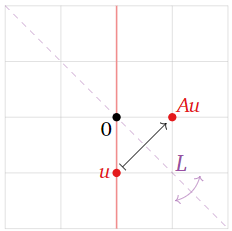
Figure \(\PageIndex{3}\)

The vector \(\color{Red}{u}\) is not an eigenvector, because \(Au\) is not collinear with \(u\) and the origin.

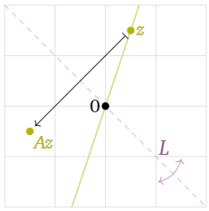
Figure \(\PageIndex{4}\)

The vector \(\color{YellowGreen}{z}\) is not an eigenvector either.

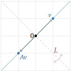
Figure \(\PageIndex{5}\)

The vector \(\color{blue}v\) is an eigenvector because \(Av\) is collinear with \(v\) and the origin. The vector \(Av\) has the same length as \(v\text{,}\) but the opposite direction, so the associated eigenvalue is \(-1\).

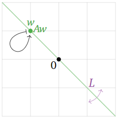
Figure \(\PageIndex{6}\)

The vector \(\color{Green}w\) is an eigenvector because \(Aw\) is collinear with \(w\) and the origin: indeed, \(Aw\) is equal to \(w\text{!}\) This means that \(w\) is an eigenvector with eigenvalue \(1\).

It appears that all eigenvectors lie either on \(L\text{,}\) or on the line perpendicular to \(L\). The vectors on \(L\) have eigenvalue \(1\text{,}\) and the vectors perpendicular to \(L\) have eigenvalue \(-1\).

Figure \(\PageIndex{7}\): An eigenvector of \(A\) is a vector \(x\) such that \(Ax\) is collinear with \(x\) and the origin. Click and drag the head of \(x\) to convince yourself that all such vectors lie either on \(L\text{,}\) or on the line perpendicular to \(L\).

We will now give five more examples of this nature

Example \(\PageIndex{5}\): Projection

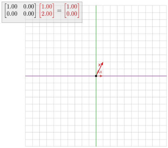
Let \(T\colon\mathbb{R}^2\to \mathbb{R}^2\) be the linear transformation that projects a vector vertically onto the \(x\)-axis, and let \(A\) be the matrix for \(T\). Find the eigenvalues and eigenvectors of \(A\) without doing any computations.

Solution

This transformation is defined geometrically, so we draw a picture.

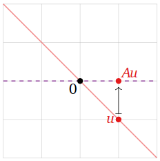
Figure \(\PageIndex{8}\)

The vector \(\color{Red}u\) is not an eigenvector, because \(Au\) is not collinear with \(u\) and the origin.

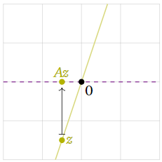
Figure \(\PageIndex{9}\)

The vector \(\color{YellowGreen}z\) is not an eigenvector either.

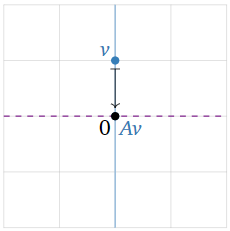
Figure \(\PageIndex{10}\)

The vector \(\color{blue}v\) is an eigenvector. Indeed, \(Av\) is the zero vector, which is collinear with \(v\) and the origin; since \(Av = 0v\text{,}\) the associated eigenvalue is \(0\).

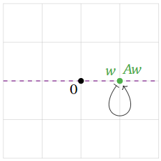
Figure \(\PageIndex{11}\)

The vector \(\color{Green}w\) is an eigenvector because \(Aw\) is collinear with \(w\) and the origin: indeed, \(Aw\) is equal to \(w\text{!}\) This means that \(w\) is an eigenvector with eigenvalue \(1\).

It appears that all eigenvectors lie on the \(x\)-axis or the \(y\)-axis. The vectors on the \(x\)-axis have eigenvalue \(1\text{,}\) and the vectors on the \(y\)-axis have eigenvalue \(0\).

Figure \(\PageIndex{12}\): An eigenvector of \(A\) is a vector \(x\) such that \(Ax\) is collinear with \(x\) and the origin. Click and drag the head of \(x\) to convince yourself that all such vectors lie on the coordinate axes.

Example \(\PageIndex{6}\): Identity

Find all eigenvalues and eigenvectors of the identity matrix \(I_n\).

Solution

The identity matrix has the property that \(I_nv = v\) for all vectors \(v\) in \(\mathbb{R}^n \). We can write this as \(I_n v = 1\cdot v\text{,}\) so every nonzero vector is an eigenvector with eigenvalue \(1\).

Figure \(\PageIndex{13}\): Every nonzero vector is an eigenvector of the identity matrix.

Example \(\PageIndex{7}\): Dilation

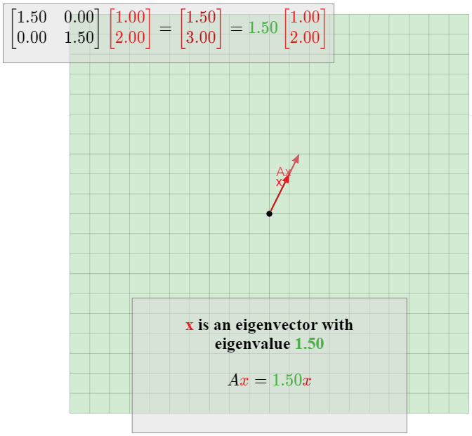
Let \(T\colon \mathbb{R} ^2\to \mathbb{R}^2\) be the linear transformation that dilates by a factor of \(1.5\text{,}\) and let \(A\) be the matrix for \(T\). Find the eigenvalues and eigenvectors of \(A\) without doing any computations.

Solution

We have

\[ Av = T(v) = 1.5v \nonumber \]

for every vector \(v\) in \(\mathbb{R}^2\). Therefore, by definition every nonzero vector is an eigenvector with eigenvalue \(1.5.\)

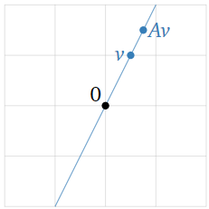
Figure \(\PageIndex{14}\)

Figure \(\PageIndex{15}\): Every nonzero vector is an eigenvector of a dilation matrix.

Example \(\PageIndex{8}\): Shear

Let

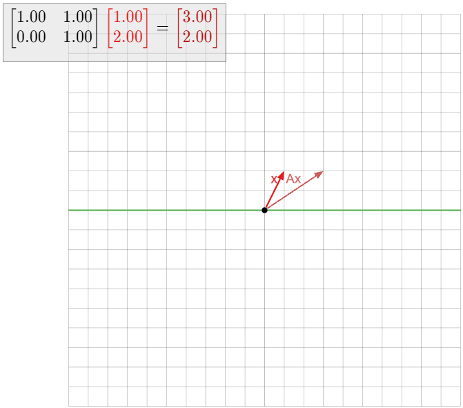
\[ A = \left(\begin{array}{cc}1&1\\0&1\end{array}\right) \nonumber \]

and let \(T(x) = Ax\text{,}\) so \(T\) is a shear in the \(x\)-direction. Find the eigenvalues and eigenvectors of \(A\) without doing any computations.

Solution

In equations, we have

\[ A\left(\begin{array}{c}x\\y\end{array}\right) = \left(\begin{array}{cc}1&1\\0&1\end{array}\right)\left(\begin{array}{c}x\\y\end{array}\right) = \left(\begin{array}{c}x+y\\y\end{array}\right). \nonumber \]

This tells us that a shear takes a vector and adds its \(y\)-coordinate to its \(x\)-coordinate. Since the \(x\)-coordinate changes but not the \(y\)-coordinate, this tells us that any vector \(v\) with nonzero \(y\)-coordinate cannot be collinear with \(Av\) and the origin.

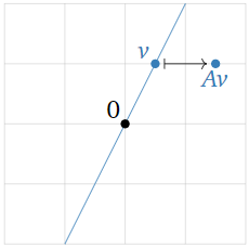
Figure \(\PageIndex{16}\)

On the other hand, any vector \(v\) on the \(x\)-axis has zero \(y\)-coordinate, so it is not moved by \(A\). Hence \(v\) is an eigenvector with eigenvalue \(1\).

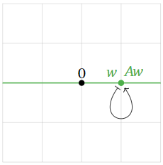
Figure \(\PageIndex{17}\)

Accordingly, all eigenvectors of \(A\) lie on the \(x\)-axis, and have eigenvalue \(1\).

Figure \(\PageIndex{18}\): All eigenvectors of a shear lie on the \(x\)-axis. Click and drag the head of \(x\) to find the eigenvectors.

Example \(\PageIndex{9}\): Rotation

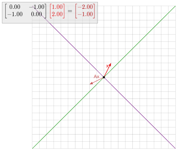
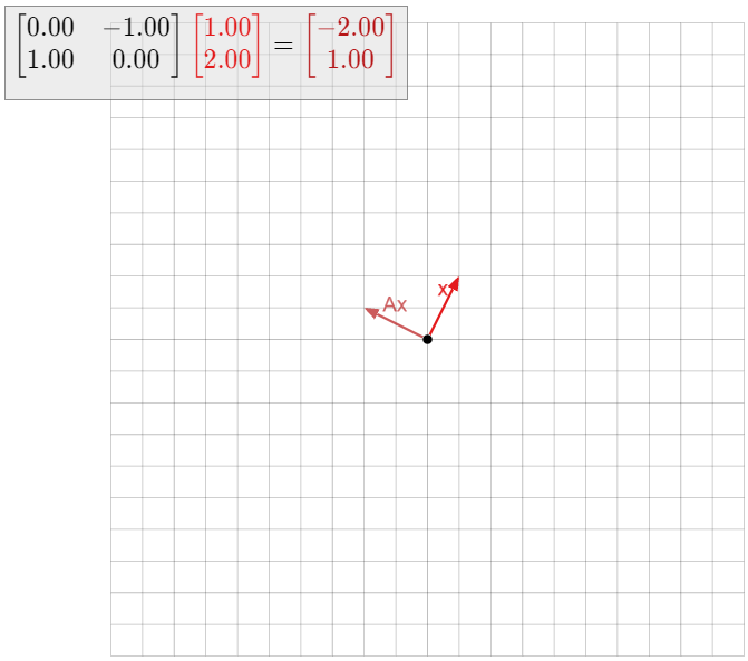
Let \(T\colon\mathbb{R}^2\to\mathbb{R}^2\) be the linear transformation that rotates counterclockwise by \(90^\circ\text{,}\) and let \(A\) be the matrix for \(T\). Find the eigenvalues and eigenvectors of \(A\) without doing any computations.

Solution

If \(v\) is any nonzero vector, then \(Av\) is rotated by an angle of \(90^\circ\) from \(v\). Therefore, \(Av\) is not on the same line as \(v\text{,}\) so \(v\) is not an eigenvector. And of course, the zero vector is never an eigenvector.

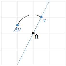
Figure \(\PageIndex{19}\)

Therefore, this matrix has no eigenvectors and eigenvalues.

Figure \(\PageIndex{20}\): This rotation matrix has no eigenvectors. Click and drag the head of \(x\) to find one.

Here we mention one basic fact about eigenvectors.

Fact \(\PageIndex{1}\): Eigenvectors with Distinct Eigenvalues are Linearly Independent

Let \(v_1,v_2,\ldots,v_k\) be eigenvectors of a matrix \(A\text{,}\) and suppose that the corresponding eigenvalues \(\lambda_1,\lambda_2,\ldots,\lambda_k\) are distinct (all different from each other). Then \(\{v_1,v_2,\ldots,v_k\}\) is linearly independent.

Proof

Suppose that \(\{v_1,v_2,\ldots,v_k\}\) were linearly dependent. According to the increasing span criterion, Theorem 2.5.2 in Section 2.5, this means that for some \(j\text{,}\) the vector \(v_j\) is in \(\text{Span}\{v_1,v_2,\ldots,v_{j-1}\}.\) If we choose the first such \(j\text{,}\) then \(\{v_1,v_2,\ldots,v_{j-1}\}\) is linearly independent. Note that \(j > 1\) since \(v_1\neq 0\).

Since \(v_j\) is in \(\text{Span}\{v_1,v_2,\ldots,v_{j-1}\},\text{,}\) we can write

\[ v_j = c_1v_1 + c_2v_2 + \cdots + c_{j-1}v_{j-1} \nonumber \]

for some scalars \(c_1,c_2,\ldots,c_{j-1}\). Multiplying both sides of the above equation by \(A\) gives

\[ \begin{split} \lambda_jv_j = Av_j \amp= A\bigl(c_1v_1 + c_2v_2 + \cdots + c_{j-1}v_{j-1}\bigr) \\ \amp= c_1Av_1 + c_2Av_2 + \cdots + c_{j-1}Av_{j-1} \\ \amp= c_1\lambda_1v_1 + c_2\lambda_2v_2 + \cdots + c_{j-1}\lambda_{j-1}v_{j-1}. \end{split} \nonumber \]

Subtracting \(\lambda_j\) times the first equation from the second gives

\[ 0 = \lambda_jv_j - \lambda_jv_j = c_1(\lambda_1-\lambda_j)v_1 + c_2(\lambda_2-\lambda_j)v_2 + \cdots + c_{j-1}(\lambda_{j-1}-\lambda_j)v_{j-1}. \nonumber \]

Since \(\lambda_i\neq\lambda_j\) for \(i \lt j\text{,}\) this is an equation of linear dependence among \(v_1,v_2,\ldots,v_{j-1}\text{,}\) which is impossible because those vectors are linearly independent. Therefore, \(\{v_1,v_2,\ldots,v_k\}\) must have been linearly independent after all.

When \(k=2\text{,}\) this says that if \(v_1,v_2\) are eigenvectors with eigenvalues \(\lambda_1\neq\lambda_2\text{,}\) then \(v_2\) is not a multiple of \(v_1\). In fact, any nonzero multiple \(cv_1\) of \(v_1\) is also an eigenvector with eigenvalue \(\lambda_1\text{:}\)

\[ A(cv_1) = cAv_1 = c(\lambda_1 v_1) = \lambda_1(cv_1). \nonumber \]

As a consequence of the above Fact \(\PageIndex{1}\), we have the following.

Note \(\PageIndex{3}\)

An \(n\times n\) matrix \(A\) has at most \(n\) eigenvalues.

Eigenspaces

Suppose that \(A\) is a square matrix. We already know how to check if a given vector is an eigenvector of \(A\) and in that case to find the eigenvalue. Our next goal is to check if a given real number is an eigenvalue of \(A\) and in that case to find all of the corresponding eigenvectors. Again this will be straightforward, but more involved. The only missing piece, then, will be to find the eigenvalues of \(A\text{;}\) this is the main content of Section 5.2.

Let \(A\) be an \(n\times n\) matrix, and let \(\lambda\) be a scalar. The eigenvectors with eigenvalue \(\lambda\text{,}\) if any, are the nonzero solutions of the equation \(Av=\lambda v\). We can rewrite this equation as follows:

\[ \begin{split} \amp Av = \lambda v \\ \iff\quad \amp Av - \lambda v = 0 \\ \iff\quad \amp Av - \lambda I_nv = 0 \\ \iff\quad \amp(A - \lambda I_n)v = 0. \end{split} \nonumber \]

Therefore, the eigenvectors of \(A\) with eigenvalue \(\lambda\text{,}\) if any, are the nontrivial solutions of the matrix equation \((A-\lambda I_n)v = 0\text{,}\) i.e., the nonzero vectors in \(\text{Nul}(A-\lambda I_n)\). If this equation has no nontrivial solutions, then \(\lambda\) is not an eigenvector of \(A\).

The above observation is important because it says that finding the eigenvectors for a given eigenvalue means solving a homogeneous system of equations. For instance, if

\[ A = \left(\begin{array}{ccc}7&1&3\\-3&2&-3\\-3&-2&-1\end{array}\right), \nonumber \]

then an eigenvector with eigenvalue \(\lambda\) is a nontrivial solution of the matrix equation

\[ \left(\begin{array}{ccc}7&1&3\\-3&2&-3\\-3&-2&-1\end{array}\right)\left(\begin{array}{c}x\\y\\z\end{array}\right) = \lambda \left(\begin{array}{c}x\\y\\z\end{array}\right). \nonumber \]

This translates to the system of equations

\[\left\{\begin{array}{rrrrrrr} 7x &+& y &+& 3z &=& \lambda x \\ -3x &+& 2y &-& 3z &=& \lambda y \\ -3x& -& 2y& -& z& =& \lambda z\end{array}\right.\quad\longrightarrow\quad\left\{\begin{array}{rrrrrrl} (7-\lambda)x &+& y &+& 3z &=& 0 \\ -3x &+& (2-\lambda)y &-& 3z &=& 0 \\ -3x& -& 2y &+& (-1-\lambda)z &=& 0.\end{array}\right.\nonumber\]

This is the same as the homogeneous matrix equation

\[ \left(\begin{array}{ccc}7-\lambda &1&3\\-3&2-\lambda&-3 \\ -3&-2&-1-\lambda\end{array}\right)\left(\begin{array}{c}x\\y\\z\end{array}\right) = 0, \nonumber \]

i.e., \((A-\lambda I_3)v = 0\).

Definition \(\PageIndex{2}\): \(\lambda\)-eigenspace

Let \(A\) be an \(n\times n\) matrix, and let \(\lambda\) be an eigenvalue of \(A\). The \(\lambda\)-eigenspace of \(A\) is the solution set of \((A-\lambda I_n)v=0\text{,}\) i.e., the subspace \(\text{Nul}(A-\lambda I_n)\).

The \(\lambda\)-eigenspace is a subspace because it is the null space of a matrix, namely, the matrix \(A-\lambda I_n\). This subspace consists of the zero vector and all eigenvectors of \(A\) with eigenvalue \(\lambda\).

Note \(\PageIndex{4}\)

Since a nonzero subspace is infinite, every eigenvalue has infinitely many eigenvectors. (For example, multiplying an eigenvector by a nonzero scalar gives another eigenvector.) On the other hand, there can be at most \(n\) linearly independent eigenvectors of an \(n\times n\) matrix, since \(\mathbb{R}^n \) has dimension \(n\).

Example \(\PageIndex{10}\): Computing eigenspaces

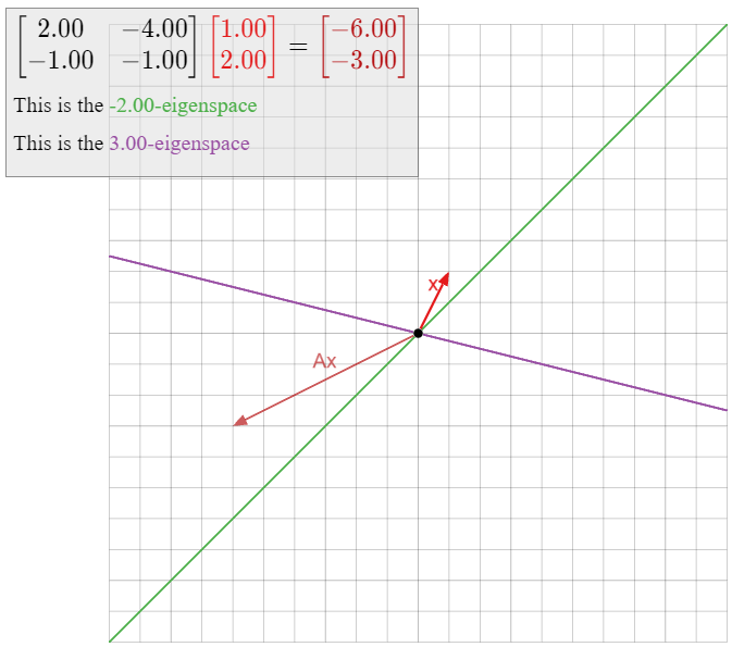
For each of the numbers \(\lambda = -2, 1, 3\text{,}\) decide if \(\lambda\) is an eigenvalue of the matrix

\[ A = \left(\begin{array}{cc}2&-4\\-1&-1\end{array}\right), \nonumber \]

and if so, compute a basis for the \(\lambda\)-eigenspace.

Solution

The number \(3\) is an eigenvalue of \(A\) if and only if \(\text{Nul}(A-3I_2)\) is nonzero. Hence, we have to solve the matrix equation \((A-3I_2)v = 0\). We have

\[ A - 3I_2 =\left(\begin{array}{cc}2&-4\\-1&-1\end{array}\right) - 3\left(\begin{array}{cc}1&0\\0&1\end{array}\right) = \left(\begin{array}{cc}-1&-4\\-1&-4\end{array}\right). \nonumber \]

The reduced row echelon form of this matrix is

\[\left(\begin{array}{cc}1&4\\0&0\end{array}\right)\quad\xrightarrow{\begin{array}{c}\text{parametric}\\ \text{form}\end{array}}\quad\left\{\begin{array}{rrr}x&=&-4y\\y&=&y\end{array}\right.\quad\xrightarrow{\begin{array}{c}\text{parametric}\\ \text{vector form}\end{array}}\quad\left(\begin{array}{c}x\\y\end{array}\right)=y\left(\begin{array}{c}-4\\1\end{array}\right).\nonumber\]

Since \(y\) is a free variable, the null space of \(A-3I_2\) is nonzero, so \(3\) is an eigenvector. A basis for the \(3\)-eigenspace is \(\bigl\{{-4\choose 1}\bigr\}.\)

Concretely, we have shown that the eigenvectors of \(A\) with eigenvalue \(3\) are exactly the nonzero multiples of \({-4\choose 1}\). In particular, \(-4\choose 1\) is an eigenvector, which we can verify:

\[\left(\begin{array}{cc}2&-4\\-1&1\end{array}\right)\left(\begin{array}{c}-4\\1\end{array}\right)=\left(\begin{array}{c}-12\\3\end{array}\right)=3\left(\begin{array}{c}-4\\1\end{array}\right).\nonumber\]

The number \(1\) is an eigenvalue of \(A\) if and only if \(\text{Nul}(A-I_2)\) is nonzero. Hence, we have to solve the matrix equation \((A-I_2)v = 0\). We have

\[A-I_{2}=\left(\begin{array}{cc}2&-4\\-1&-1\end{array}\right)-\left(\begin{array}{cc}1&0\\0&1\end{array}\right)=\left(\begin{array}{cc}1&-4\\-1&-2\end{array}\right).\nonumber\]

This matrix has determinant \(-6\text{,}\) so it is invertible. By Theorem 3.6.1 in Section 3.6, we have \(\text{Nul}(A-I_2) = \{0\}\text{,}\) so \(1\) is not an eigenvalue.

The eigenvectors of \(A\) with eigenvalue \(-2\text{,}\) if any, are the nonzero solutions of the matrix equation \((A+2I_2)v = 0\). We have

\[A+2I_{2}=\left(\begin{array}{cc}2&-4\\-1&-1\end{array}\right)+2\left(\begin{array}{cc}1&0\\0&1\end{array}\right)=\left(\begin{array}{cc}4&-4\\-1&1\end{array}\right).\nonumber\]

The reduced row echelon form of this matrix is

\[\left(\begin{array}{cc}1&-1\\0&0\end{array}\right)\quad\xrightarrow{\begin{array}{c}\text{parametric}\\ \text{form}\end{array}}\quad\left\{\begin{array}{rrr}x&=&y\\y&=&y\end{array}\right.\quad\xrightarrow{\begin{array}{c}\text{parametric}\\ \text{vector form}\end{array}}\quad\left(\begin{array}{c}x\\y\end{array}\right)=y\left(\begin{array}{c}1\\1\end{array}\right).\nonumber\]

Hence there exist eigenvectors with eigenvalue \(-2\text{,}\) namely, any nonzero multiple of \({1\choose 1}.\) A basis for the \(-2\)-eigenspace is \(\bigl\{{1\choose 1}\bigr\}.\)

Figure \(\PageIndex{21}\): The \(3\)-eigenspace is the line spanned by \({-4\choose 1}.\) This means that \(A\) scales every vector in that line by a factor of \(3\). Likewise, the \(-2\)-eigenspace is the line spanned by \({1\choose 1}.\) Click and drag the vector \(x\) around to see how \(A\) acts on that vector.

Example \(\PageIndex{11}\): Computing eigenspaces

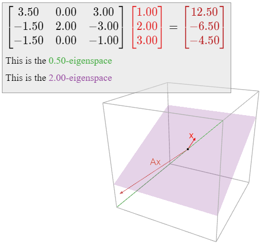
For each of the numbers \(\lambda=0, \frac 12, 2\text{,}\) decide if \(\lambda\) is an eigenvector of the matrix

\[A=\left(\begin{array}{ccc}7/2&0&3\\ -3/2&2&-3\\ -3/2&0&-1\end{array}\right),\nonumber\]

and if so, compute a basis for the \(\lambda\)-eigenspace.

Solution

The number \(2\) is an eigenvalue of \(A\) if and only if \(\text{Nul}(A-2I_3)\) is nonzero. Hence, we have to solve the matrix equation \((A-2I_3)v = 0\). We have

\[A-2I_{3}=\left(\begin{array}{ccc}7/2&0&3 \\ -3/2&2&-3\\ -3/2&0&1\end{array}\right) -2\left(\begin{array}{ccc}1&0&0\\0&1&0\\0&0&1\end{array}\right)=\left(\begin{array}{ccc}3/2&0&3 \\ -3/2&0&-3\\ -3/2&0&-3\end{array}\right).\nonumber\]

The reduced row echelon form of this matrix is

\[\left(\begin{array}{ccc}1&0&2\\0&0&0\\0&0&0\end{array}\right)\quad\xrightarrow{\begin{array}{c}\text{parametric} \\ \text{form}\end{array}}\quad\left\{\begin{array}{rrr}x&=&-2z \\ y&=&y \\ z&=&z\end{array}\right.\quad\xrightarrow{\begin{array}{c}\text{parametric}\\ \text{vector form}\end{array}}\quad\left(\begin{array}{c}x\\y\\z\end{array}\right)=y\left(\begin{array}{c}0\\1\\0\end{array}\right)+z\left(\begin{array}{c}-2\\0\\1\end{array}\right).\nonumber\]

The matrix \(A-2I_3\) has two free variables, so the null space of \(A-2I_3\) is nonzero, and thus \(2\) is an eigenvector. A basis for the \(2\)-eigenspace is

\[ \left\{\left(\begin{array}{c}0\\1\\0\end{array}\right),\,\left(\begin{array}{c}-2\\0\\1\end{array}\right)\right\}. \nonumber \]

This is a plane in \(\mathbb{R}^3 \).

The eigenvectors of \(A\) with eigenvalue \(\frac 12\text{,}\) if any, are the nonzero solutions of the matrix equation \((A-\frac 12I_3)v = 0\). We have

\[A-\frac{1}{2}I_{3}=\left(\begin{array}{ccc}7/2&0&3\\ -3/2&2&-3\\ -3/2&0&1\end{array}\right)-\frac{1}{2}\left(\begin{array}{ccc}1&0&0\\0&1&0\\0&0&1\end{array}\right)=\left(\begin{array}{ccc}3&0&3\\-3/2&3/2&-3 \\ -3/2&0&-3/2\end{array}\right).\nonumber\]

The reduced row echelon form of this matrix is

\[\left(\begin{array}{ccc}1&0&1\\0&1&-1\\0&0&0\end{array}\right)\quad\xrightarrow{\begin{array}{c}\text{parametric}\\ \text{form}\end{array}}\quad\left\{\begin{array}{rrr}x&=&-z\\ y&=&z \\ z&=&z\end{array}\right.\quad\xrightarrow{\begin{array}{c}\text{parametric} \\ \text{vector form}\end{array}}\quad\left(\begin{array}{c}x\\y\\z\end{array}\right)=z\left(\begin{array}{c}-1\\1\\1\end{array}\right).\nonumber\]

Hence there exist eigenvectors with eigenvalue \(\frac 12\text{,}\) so \(\frac 12\) is an eigenvalue. A basis for the \(\frac 12\)-eigenspace is

\[ \left\{\left(\begin{array}{c}-1\\1\\1\end{array}\right)\right\}. \nonumber \]

This is a line in \(\mathbb{R}^3 \).

The number \(0\) is an eigenvalue of \(A\) if and only if \(\text{Nul}(A-0I_3) = \text{Nul}(A)\) is nonzero. This is the same as asking whether \(A\) is noninvertible, by Theorem 3.6.1 in Section 3.6. The determinant of \(A\) is \(\det(A) = 2\neq 0\text{,}\) so \(A\) is invertible by the invertibility property, Proposition 4.1.2 in Section 4.1. It follows that \(0\) is not an eigenvalue of \(A\).

Figure \(\PageIndex{22}\): The \(2\)-eigenspace is the violet plane. This means that \(A\) scales every vector in that plane by a factor of \(2\). The \(\frac 12\)-eigenspace is the green line. Click and drag the vector \(x\) around to see how \(A\) acts on that vector.

Example \(\PageIndex{12}\): Reflection

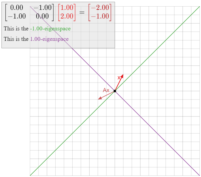
Let \(T\colon\mathbb{R}^2\to\mathbb{R}^2\) be the linear transformation that reflects over the line \(L\) defined by \(y=-x\text{,}\) and let \(A\) be the matrix for \(T\). Find all eigenspaces of \(A\).

Solution

We showed in Example \(\PageIndex{4}\) that all eigenvectors with eigenvalue \(1\) lie on \(L\text{,}\) and all eigenvectors with eigenvalue \(-1\) lie on the line \(L^\perp\) that is perpendicular to \(L\). Hence, \(L\) is the \(1\)-eigenspace, and \(L^\perp\) is the \(-1\)-eigenspace.

None of this required any computations, but we can verify our conclusions using algebra. First we compute the matrix \(A\text{:}\)

\[T\left(\begin{array}{c}1\\0\end{array}\right)=\left(\begin{array}{c}0\\-1\end{array}\right)\quad T\left(\begin{array}{c}0\\1\end{array}\right)=\left(\begin{array}{c}-1\\0\end{array}\right)\quad\implies\quad A=\left(\begin{array}{cc}0&-1\\-1&0\end{array}\right).\nonumber\]

Computing the \(1\)-eigenspace means solving the matrix equation \((A-I_2)v=0\). We have

\[A-I_{2}=\left(\begin{array}{cc}0&-1\\-1&0\end{array}\right)-\left(\begin{array}{cc}1&0\\0&1\end{array}\right)=\left(\begin{array}{cc}-1&-1\\-1&-1\end{array}\right)\quad\xrightarrow{\text{RREF}}\quad\left(\begin{array}{cc}1&1\\0&0\end{array}\right).\nonumber\]

The parametric form of the solution set is \(x = -y\text{,}\) or equivalently, \(y = -x\text{,}\) which is exactly the equation for \(L\). Computing the \(-1\)-eigenspace means solving the matrix equation \((A+I_2)v=0\text{;}\) we have

\[A+I_{2}=\left(\begin{array}{cc}0&-1\\-1&0\end{array}\right)+\left(\begin{array}{cc}1&0\\0&1\end{array}\right)=\left(\begin{array}{cc}1&-1\\-1&1\end{array}\right)\quad\xrightarrow{\text{RREF}}\quad\left(\begin{array}{cc}1&-1\\0&0\end{array}\right).\nonumber\]

The parametric form of the solution set is \(x = y\text{,}\) or equivalently, \(y = x\text{,}\) which is exactly the equation for \(L^\perp\).

Figure \(\PageIndex{23}\): The violet line \(L\) is the \(1\)-eigenspace, and the green line \(L^\perp\) is the \(-1\)-eigenspace.

Recipe: Eigenspaces

Let \(A\) be an \(n\times n\) matrix and let \(\lambda\) be a number.

1. \(\lambda\) is an eigenvalue of \(A\) if and only if \((A-\lambda I_n)v = 0\) has a nontrivial solution, if and only if \(\text{Nul}(A-\lambda I_n)\neq\{0\}.\)
2. In this case, finding a basis for the \(\lambda\)-eigenspace of \(A\) means finding a basis for \(\text{Nul}(A-\lambda I_n)\text{,}\) which can be done by finding the parametric vector form of the solutions of the homogeneous system of equations \((A-\lambda I_n)v = 0\).
3. The dimension of the \(\lambda\)-eigenspace of \(A\) is equal to the number of free variables in the system of equations \((A-\lambda I_n)v = 0\text{,}\) which is the number of columns of \(A - \lambda I_n\) without pivots.
4. The eigenvectors with eigenvalue \(\lambda\) are the nonzero vectors in \(\text{Nul}(A-\lambda I_n),\) or equivalently, the nontrivial solutions of \((A-\lambda I_n)v = 0\).

We conclude with an observation about the \(0\)-eigenspace of a matrix.

Fact \(\PageIndex{2}\)

Let \(A\) be an \(n\times n\) matrix.

1. The number \(0\) is an eigenvalue of \(A\) if and only if \(A\) is not invertible.
2. In this case, the \(0\)-eigenspace of \(A\) is \(\text{Nul}(A)\).

Proof

We know that \(0\) is an eigenvalue of \(A\) if and only if \(\text{Nul}(A - 0I_n) = \text{Nul}(A)\) is nonzero, which is equivalent to the noninvertibility of \(A\) by Theorem 3.6.1 in Section 3.6. In this case, the \(0\)-eigenspace is by definition \(\text{Nul}(A-0I_n) = \text{Nul}(A)\).

Concretely, an eigenvector with eigenvalue \(0\) is a nonzero vector \(v\) such that \(Av=0v\text{,}\) i.e., such that \(Av = 0\). These are exactly the nonzero vectors in the null space of \(A\).

The Invertible Matrix Theorem: Addenda

We now have two new ways of saying that a matrix is invertible, so we add them to the invertible matrix theorem, Theorem 3.6.1 in Section 3.6.

Theorem \(\PageIndex{1}\): Invertible Matrix Theorem

Let \(A\) be an \(n\times n\) matrix, and let \(T\colon\mathbb{R}^n \to\mathbb{R}^n \) be the matrix transformation \(T(x) = Ax\). The following statements are equivalent:

1. \(A\) is invertible.
2. \(A\) has \(n\) pivots.
3. \(\text{Nul}(A) = \{0\}\).
4. The columns of \(A\) are linearly independent.
5. The columns of \(A\) span \(\mathbb{R}^n \).
6. \(Ax=b\) has a unique solution for each \(b\) in \(\mathbb{R}^n \).
7. \(T\) is invertible.
8. \(T\) is one-to-one.
9. \(T\) is onto.
10. \(\det(A) \neq 0\).
11. \(0\) is not an eigenvalue of \(A\).