
4.1: Determinants- Definition
- Page ID
- 70202

\( \newcommand{\vecs}[1]{\overset { \scriptstyle \rightharpoonup} {\mathbf{#1}} } \)
\( \newcommand{\vecd}[1]{\overset{-\!-\!\rightharpoonup}{\vphantom{a}\smash {#1}}} \)
\( \newcommand{\dsum}{\displaystyle\sum\limits} \)
\( \newcommand{\dint}{\displaystyle\int\limits} \)
\( \newcommand{\dlim}{\displaystyle\lim\limits} \)
\( \newcommand{\id}{\mathrm{id}}\) \( \newcommand{\Span}{\mathrm{span}}\)
( \newcommand{\kernel}{\mathrm{null}\,}\) \( \newcommand{\range}{\mathrm{range}\,}\)
\( \newcommand{\RealPart}{\mathrm{Re}}\) \( \newcommand{\ImaginaryPart}{\mathrm{Im}}\)
\( \newcommand{\Argument}{\mathrm{Arg}}\) \( \newcommand{\norm}[1]{\| #1 \|}\)
\( \newcommand{\inner}[2]{\langle #1, #2 \rangle}\)
\( \newcommand{\Span}{\mathrm{span}}\)
\( \newcommand{\id}{\mathrm{id}}\)
\( \newcommand{\Span}{\mathrm{span}}\)
\( \newcommand{\kernel}{\mathrm{null}\,}\)
\( \newcommand{\range}{\mathrm{range}\,}\)
\( \newcommand{\RealPart}{\mathrm{Re}}\)
\( \newcommand{\ImaginaryPart}{\mathrm{Im}}\)
\( \newcommand{\Argument}{\mathrm{Arg}}\)
\( \newcommand{\norm}[1]{\| #1 \|}\)
\( \newcommand{\inner}[2]{\langle #1, #2 \rangle}\)
\( \newcommand{\Span}{\mathrm{span}}\) \( \newcommand{\AA}{\unicode[.8,0]{x212B}}\)
\( \newcommand{\vectorA}[1]{\vec{#1}} % arrow\)
\( \newcommand{\vectorAt}[1]{\vec{\text{#1}}} % arrow\)
\( \newcommand{\vectorB}[1]{\overset { \scriptstyle \rightharpoonup} {\mathbf{#1}} } \)
\( \newcommand{\vectorC}[1]{\textbf{#1}} \)
\( \newcommand{\vectorD}[1]{\overrightarrow{#1}} \)
\( \newcommand{\vectorDt}[1]{\overrightarrow{\text{#1}}} \)
\( \newcommand{\vectE}[1]{\overset{-\!-\!\rightharpoonup}{\vphantom{a}\smash{\mathbf {#1}}}} \)
\( \newcommand{\vecs}[1]{\overset { \scriptstyle \rightharpoonup} {\mathbf{#1}} } \)
\(\newcommand{\longvect}{\overrightarrow}\)
\( \newcommand{\vecd}[1]{\overset{-\!-\!\rightharpoonup}{\vphantom{a}\smash {#1}}} \)
\(\newcommand{\avec}{\mathbf a}\) \(\newcommand{\bvec}{\mathbf b}\) \(\newcommand{\cvec}{\mathbf c}\) \(\newcommand{\dvec}{\mathbf d}\) \(\newcommand{\dtil}{\widetilde{\mathbf d}}\) \(\newcommand{\evec}{\mathbf e}\) \(\newcommand{\fvec}{\mathbf f}\) \(\newcommand{\nvec}{\mathbf n}\) \(\newcommand{\pvec}{\mathbf p}\) \(\newcommand{\qvec}{\mathbf q}\) \(\newcommand{\svec}{\mathbf s}\) \(\newcommand{\tvec}{\mathbf t}\) \(\newcommand{\uvec}{\mathbf u}\) \(\newcommand{\vvec}{\mathbf v}\) \(\newcommand{\wvec}{\mathbf w}\) \(\newcommand{\xvec}{\mathbf x}\) \(\newcommand{\yvec}{\mathbf y}\) \(\newcommand{\zvec}{\mathbf z}\) \(\newcommand{\rvec}{\mathbf r}\) \(\newcommand{\mvec}{\mathbf m}\) \(\newcommand{\zerovec}{\mathbf 0}\) \(\newcommand{\onevec}{\mathbf 1}\) \(\newcommand{\real}{\mathbb R}\) \(\newcommand{\twovec}[2]{\left[\begin{array}{r}#1 \\ #2 \end{array}\right]}\) \(\newcommand{\ctwovec}[2]{\left[\begin{array}{c}#1 \\ #2 \end{array}\right]}\) \(\newcommand{\threevec}[3]{\left[\begin{array}{r}#1 \\ #2 \\ #3 \end{array}\right]}\) \(\newcommand{\cthreevec}[3]{\left[\begin{array}{c}#1 \\ #2 \\ #3 \end{array}\right]}\) \(\newcommand{\fourvec}[4]{\left[\begin{array}{r}#1 \\ #2 \\ #3 \\ #4 \end{array}\right]}\) \(\newcommand{\cfourvec}[4]{\left[\begin{array}{c}#1 \\ #2 \\ #3 \\ #4 \end{array}\right]}\) \(\newcommand{\fivevec}[5]{\left[\begin{array}{r}#1 \\ #2 \\ #3 \\ #4 \\ #5 \\ \end{array}\right]}\) \(\newcommand{\cfivevec}[5]{\left[\begin{array}{c}#1 \\ #2 \\ #3 \\ #4 \\ #5 \\ \end{array}\right]}\) \(\newcommand{\mattwo}[4]{\left[\begin{array}{rr}#1 \amp #2 \\ #3 \amp #4 \\ \end{array}\right]}\) \(\newcommand{\laspan}[1]{\text{Span}\{#1\}}\) \(\newcommand{\bcal}{\cal B}\) \(\newcommand{\ccal}{\cal C}\) \(\newcommand{\scal}{\cal S}\) \(\newcommand{\wcal}{\cal W}\) \(\newcommand{\ecal}{\cal E}\) \(\newcommand{\coords}[2]{\left\{#1\right\}_{#2}}\) \(\newcommand{\gray}[1]{\color{gray}{#1}}\) \(\newcommand{\lgray}[1]{\color{lightgray}{#1}}\) \(\newcommand{\rank}{\operatorname{rank}}\) \(\newcommand{\row}{\text{Row}}\) \(\newcommand{\col}{\text{Col}}\) \(\renewcommand{\row}{\text{Row}}\) \(\newcommand{\nul}{\text{Nul}}\) \(\newcommand{\var}{\text{Var}}\) \(\newcommand{\corr}{\text{corr}}\) \(\newcommand{\len}[1]{\left|#1\right|}\) \(\newcommand{\bbar}{\overline{\bvec}}\) \(\newcommand{\bhat}{\widehat{\bvec}}\) \(\newcommand{\bperp}{\bvec^\perp}\) \(\newcommand{\xhat}{\widehat{\xvec}}\) \(\newcommand{\vhat}{\widehat{\vvec}}\) \(\newcommand{\uhat}{\widehat{\uvec}}\) \(\newcommand{\what}{\widehat{\wvec}}\) \(\newcommand{\Sighat}{\widehat{\Sigma}}\) \(\newcommand{\lt}{<}\) \(\newcommand{\gt}{>}\) \(\newcommand{\amp}{&}\) \(\definecolor{fillinmathshade}{gray}{0.9}\)- Learn the definition of the determinant.
- Learn some ways to eyeball a matrix with zero determinant, and how to compute determinants of upper- and lower-triangular matrices.
- Learn the basic properties of the determinant, and how to apply them.
- Recipe: compute the determinant using row and column operations.
- Theorems: existence theorem, invertibility property, multiplicativity property, transpose property.
- Vocabulary words: diagonal, upper-triangular, lower-triangular, transpose.
- Essential vocabulary word: determinant.
In this section, we define the determinant, and we present one way to compute it. Then we discuss some of the many wonderful properties the determinant enjoys.
The Definition of the Determinant
The determinant of a square matrix \(A\) is a real number \(\det(A)\). It is defined via its behavior with respect to row operations; this means we can use row reduction to compute it. We will give a recursive formula for the determinant in Section 4.2. We will also show in Subsection Magical Properties of the Determinant that the determinant is related to invertibility, and in Section 4.3 that it is related to volumes.
The determinant is a function
\[ \det\colon \bigl\{\text{square matrices}\bigr\}\to \mathbb{R} \nonumber \]
satisfying the following properties:
- Doing a row replacement on \(A\) does not change \(\det(A)\).
- Scaling a row of \(A\) by a scalar \(c\) multiplies the determinant by \(c\).
- Swapping two rows of a matrix multiplies the determinant by \(-1\).
- The determinant of the identity matrix \(I_n\) is equal to \(1\).
In other words, to every square matrix \(A\) we assign a number \(\det(A)\) in a way that satisfies the above properties.
In each of the first three cases, doing a row operation on a matrix scales the determinant by a nonzero number. (Multiplying a row by zero is not a row operation.) Therefore, doing row operations on a square matrix \(A\) does not change whether or not the determinant is zero.
The main motivation behind using these particular defining properties is geometric: see Section 4.3. Another motivation for this definition is that it tells us how to compute the determinant: we row reduce and keep track of the changes.
Let us compute \(\det\left(\begin{array}{cc}2&1\\1&4\end{array}\right).\) First we row reduce, then we compute the determinant in the opposite order:
\begin{align*} \amp\left(\begin{array}{cc}2&1\\1&4\end{array}\right) \amp\strut\det\amp=7\\ \;\xrightarrow{R_1\leftrightarrow R_2}\;\amp \left(\begin{array}{cc}1&4\\2&1\end{array}\right) \amp \strut\det \amp= -7\\ \;\xrightarrow{R_2=R_2-2R_1}\;\amp \left(\begin{array}{cc}1&4\\0&-7\end{array}\right) \amp \strut\det \amp= -7\\ \;\xrightarrow{R_2=R_2\div -7}\;\amp \left(\begin{array}{cc}1&4\\0&1\end{array}\right) \amp \strut\det \amp= 1\\ \;\xrightarrow{R_1=R_1-4R_2}\;\amp \left(\begin{array}{cc}1&0\\0&1\end{array}\right) \amp \strut\det \amp= 1 \end{align*}
The reduced row echelon form of the matrix is the identity matrix \(I_2\text{,}\) so its determinant is \(1\). The second-last step in the row reduction was a row replacement, so the second-final matrix also has determinant \(1\). The previous step in the row reduction was a row scaling by \(-1/7\text{;}\) since (the determinant of the second matrix times \(-1/7\)) is \(1\text{,}\) the determinant of the second matrix must be \(-7\). The first step in the row reduction was a row swap, so the determinant of the first matrix is negative the determinant of the second. Thus, the determinant of the original matrix is \(7\).
Note that our answer agrees with Definition 3.5.2 in Section 3.5 of the determinant.
Compute \(\det\left(\begin{array}{cc}1&0\\0&3\end{array}\right)\).
Solution
Let \(A=\left(\begin{array}{cc}1&0\\0&3\end{array}\right)\). Since \(A\) is obtained from \(I_2\) by multiplying the second row by the constant \(3\text{,}\) we have
\[ \det(A)=3\det(I_2)=3\cdot 1=3. \nonumber \]
Note that our answer agrees with Definition 3.5.2 in Section 3.5 of the determinant.
Compute \(\det\left(\begin{array}{ccc}1&0&0\\0&0&1\\5&1&0\end{array}\right)\).
Solution
First we row reduce, then we compute the determinant in the opposite order:
\begin{align*} \amp\left(\begin{array}{ccc}1&0&0\\0&0&1\\5&1&0\end{array}\right) \amp\strut\det\amp=-1\\ \;\xrightarrow{R_2\leftrightarrow R_3}\;\amp \left(\begin{array}{ccc}1&0&0\\5&1&0\\0&0&1\end{array}\right) \amp \strut\det \amp= 1\\ \;\xrightarrow{R_2=R_2-5R_1}\;\amp \left(\begin{array}{ccc}1&0&0\\0&1&0\\0&0&1\end{array}\right) \amp \strut\det \amp= 1 \end{align*}
The reduced row echelon form is \(I_3\text{,}\) which has determinant \(1\). Working backwards from \(I_3\) and using the four defining properties Definition \(\PageIndex{1}\), we see that the second matrix also has determinant \(1\) (it differs from \(I_3\) by a row replacement), and the first matrix has determinant \(-1\) (it differs from the second by a row swap).
Here is the general method for computing determinants using row reduction.
Let \(A\) be a square matrix. Suppose that you do some number of row operations on \(A\) to obtain a matrix \(B\) in row echelon form. Then
\[ \det(A) = (-1)^r\cdot \frac{\text{(product of the diagonal entries of $B$)}} {\text{(product of scaling factors used)}}, \nonumber \]
where \(r\) is the number of row swaps performed.
In other words, the determinant of \(A\) is the product of diagonal entries of the row echelon form \(B\text{,}\) times a factor of \(\pm1\) coming from the number of row swaps you made, divided by the product of the scaling factors used in the row reduction.
This is an efficient way of computing the determinant of a large matrix, either by hand or by computer. The computational complexity of row reduction is \(O(n^3)\text{;}\) by contrast, the cofactor expansion algorithm we will learn in Section 4.2 has complexity \(O(n!)\approx O(n^n\sqrt n)\text{,}\) which is much larger. (Cofactor expansion has other uses.)
Compute \(\det\left(\begin{array}{ccc}0&-7&-4\\2&4&6\\3&7&-1\end{array}\right).\)
Solution
We row reduce the matrix, keeping track of the number of row swaps and of the scaling factors used.
\[\begin{aligned}\left(\begin{array}{ccc}0&-7&-4\\2&4&6\\3&7&-1\end{array}\right)\quad\xrightarrow{R_1\leftrightarrow R_2}\quad &\left(\begin{array}{ccc}2&4&6\\0&-7&-4\\3&7&-1\end{array}\right)\quad r=1 \\ {}\xrightarrow{R_1=R_1\div 2}\quad &\left(\begin{array}{ccc}1&2&3\\0&-7&-4\\3&7&-1\end{array}\right)\quad \text{scaling factors }=\frac{1}{2} \\ {}\xrightarrow{R_3=R_3-3R_1}\quad &\left(\begin{array}{ccc}1&2&3\\0&-7&-4\\0&1&-10\end{array}\right) \\ {}\xrightarrow{R_2\leftrightarrow R_3}\quad &\left(\begin{array}{ccc}1&2&3\\0&1&-10\\0&-7&-4\end{array}\right)\quad r=2 \\ {}\xrightarrow{R_3=R_3+7R_2}\quad &\left(\begin{array}{c}1&2&3\\0&1&-10\\0&0&-74\end{array}\right)\end{aligned}\]
We made two row swaps and scaled once by a factor of \(1/2\text{,}\) so the Recipe: Computing Determinants by Row Reducing says that
\[ \det\left(\begin{array}{ccc}0&-7&-4\\2&4&6\\3&7&-1\end{array}\right) = (-1)^2\cdot\frac{1\cdot 1\cdot(-74)}{1/2} = -148. \nonumber \]
Compute \(\det\left(\begin{array}{ccc}1&2&3\\2&-1&1\\3&0&1\end{array}\right).\)
Solution
We row reduce the matrix, keeping track of the number of row swaps and of the scaling factors used.
\[\begin{aligned}\left(\begin{array}{ccc}1&2&3\\2&-1&1\\3&0&1\end{array}\right)\quad\xrightarrow{\begin{array}{l}{R_2=R_2-2R_1}\\{R_3=R_3-3R_1}\end{array}}\quad &\left(\begin{array}{ccc}1&2&3\\0&-5&-5 \\ 0&-6&-8\end{array}\right) \\ {}\xrightarrow{R_2=R_2\div 5}\quad &\left(\begin{array}{ccc}1&2&3\\0&1&1\\0&-6&-8\end{array}\right)\quad\text{scaling factors }=-\frac{1}{5} \\ {}\xrightarrow{R_3=R_3+6R_2}\quad &\left(\begin{array}{ccc}1&2&3\\0&1&1\\0&0&-2\end{array}\right)\end{aligned}\]
We did not make any row swaps, and we scaled once by a factor of \(-1/5\text{,}\) so the Recipe: Computing Determinants by Row Reducing says that
\[ \det\left(\begin{array}{ccc}1&2&3\\2&-1&1\\3&0&1\end{array}\right) = \frac{1\cdot 1\cdot(-2)}{-1/5} = 10. \nonumber \]
Let us use the Recipe: Computing Determinants by Row Reducing to compute the determinant of a general \(2\times 2\) matrix \(A = \left(\begin{array}{cc}a&b\\c&d\end{array}\right)\).
- If \(a = 0\text{,}\) then
\[ \det\left(\begin{array}{cc}a&b\\c&d\end{array}\right) = \det\left(\begin{array}{cc}0&b\\c&d\end{array}\right) = -\det\left(\begin{array}{cc}c&d\\0&b\end{array}\right) = -bc. \nonumber \] - If \(a\neq 0\text{,}\) then
\[\begin{aligned} \det\left(\begin{array}{cc}a&b\\c&d\end{array}\right)&=a\cdot\det\left(\begin{array}{cc}1&b/a\\c&d\end{array}\right)=a\cdot\det\left(\begin{array}{cc}1&b/a \\ 0&d-c\cdot b/a\end{array}\right) \\ &=a\cdot 1\cdot (d-bc/a)=ad-bc.\end{aligned}\]
In either case, we recover Definition 3.5.2 in Section 3.5.
\[ \det\left(\begin{array}{cc}a&b\\c&d\end{array}\right) = ad-bc. \nonumber \]
If a matrix is already in row echelon form, then you can simply read off the determinant as the product of the diagonal entries. It turns out this is true for a slightly larger class of matrices called triangular.
- The diagonal entries of a matrix \(A\) are the entries \(a_{11},a_{22},\ldots\text{:}\)
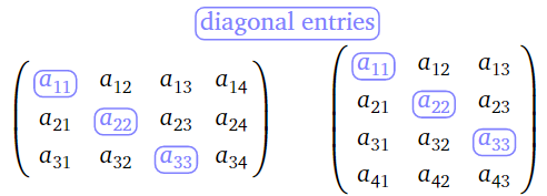
Figure \(\PageIndex{1}\)
- A square matrix is called upper-triangular if its nonzero entries all lie above the diagonal, and it is called lower-triangular if its nonzero entries all lie below the diagonal. It is called diagonal if all of its nonzero entries lie on the diagonal, i.e., if it is both upper-triangular and lower-triangular.
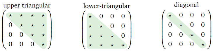
Figure \(\PageIndex{2}\)
Let \(A\) be an \(n\times n\) matrix.
- If \(A\) has a zero row or column, then \(\det(A) = 0.\)
- If \(A\) is upper-triangular or lower-triangular, then \(\det(A)\) is the product of its diagonal entries.
- Proof
-
- Suppose that \(A\) has a zero row. Let \(B\) be the matrix obtained by negating the zero row. Then \(\det(A) = -\det(B)\) by the second defining property, Definition \(\PageIndex{1}\). But \(A = B\text{,}\) so \(\det(A) = \det(B)\text{:}\)
\[\left(\begin{array}{ccc}1&2&3\\0&0&0\\7&8&9\end{array}\right)\quad\xrightarrow{R_2=-R_2}\quad\left(\begin{array}{ccc}1&2&3\\0&0&0\\7&8&9\end{array}\right).\nonumber\]
Putting these together yields \(\det(A) = -\det(A)\text{,}\) so \(\det(A)=0\).
Now suppose that \(A\) has a zero column. Then \(A\) is not invertible by Theorem 3.6.1 in Section 3.6, so its reduced row echelon form has a zero row. Since row operations do not change whether the determinant is zero, we conclude \(\det(A)=0\). - First suppose that \(A\) is upper-triangular, and that one of the diagonal entries is zero, say \(a_{ii}=0\). We can perform row operations to clear the entries above the nonzero diagonal entries:
\[\left(\begin{array}{cccc}a_{11}&\star&\star&\star \\ 0&a_{22}&\star&\star \\ 0&0&0&\star \\ 0&0&0&a_{44}\end{array}\right)\xrightarrow{\qquad}\left(\begin{array}{cccc}a_{11}&0&\star &0\\0&a_{22}&\star&0\\0&0&0&0\\0&0&0&a_{44}\end{array}\right)\nonumber\]
In the resulting matrix, the \(i\)th row is zero, so \(\det(A) = 0\) by the first part.
Still assuming that \(A\) is upper-triangular, now suppose that all of the diagonal entries of \(A\) are nonzero. Then \(A\) can be transformed to the identity matrix by scaling the diagonal entries and then doing row replacements:
\[\begin{array}{ccccc}{\left(\begin{array}{ccc}a&\star&\star \\ 0&b&\star \\ 0&0&c\end{array}\right)}&{\xrightarrow{\begin{array}{c}{\text{scale by}}\\{a^{-1},\:b^{-1},\:c^{-1}}\end{array}}}&{\left(\begin{array}{ccc}1&\star&\star \\ 0&1&\star \\ 0&0&1\end{array}\right)}&{\xrightarrow{\begin{array}{c}{\text{row}}\\{\text{replacements}}\end{array}}}&{\left(\begin{array}{ccc}1&0&0\\0&1&0\\0&0&1\end{array}\right)}\\{\det =abc}&{\xleftarrow{\qquad}}&{\det =1}&{\xleftarrow{\qquad}}&{\det =1}\end{array}\nonumber\]
Since \(\det(I_n) = 1\) and we scaled by the reciprocals of the diagonal entries, this implies \(\det(A)\) is the product of the diagonal entries.
The same argument works for lower triangular matrices, except that the the row replacements go down instead of up.
- Suppose that \(A\) has a zero row. Let \(B\) be the matrix obtained by negating the zero row. Then \(\det(A) = -\det(B)\) by the second defining property, Definition \(\PageIndex{1}\). But \(A = B\text{,}\) so \(\det(A) = \det(B)\text{:}\)
Compute the determinants of these matrices:
\[\left(\begin{array}{ccc}1&2&3\\0&4&5\\0&0&6\end{array}\right)\qquad\left(\begin{array}{ccc}-20&0&0\\ \pi&0&0\\ 100&3&-7\end{array}\right)\qquad\left(\begin{array}{ccc}17&03&4\\0&0&0\\11/2&1&e\end{array}\right).\nonumber\]
Solution
The first matrix is upper-triangular, the second is lower-triangular, and the third has a zero row:
\[\begin{aligned}\det\left(\begin{array}{ccc}1&2&3\\0&4&5\\0&0&6\end{array}\right)&=1\cdot 4\cdot 6=24 \\ \det\left(\begin{array}{ccc}-20&0&0\\ \pi&0&0\\100&3&-7\end{array}\right)&=-20\cdot 0\cdot -7=0 \\ \det\left(\begin{array}{ccc}17&-3&4\\0&0&0\\ 11/2&1&e\end{array}\right)&=0.\end{aligned}\]
A matrix can always be transformed into row echelon form by a series of row operations, and a matrix in row echelon form is upper-triangular. Therefore, we have completely justified Recipe: Computing Determinants by Row Reducing for computing the determinant.
The determinant is characterized by its defining properties, Definition \(\PageIndex{1}\), since we can compute the determinant of any matrix using row reduction, as in the above Recipe: Computing Determinants by Row Reducing. However, we have not yet proved the existence of a function satisfying the defining properties! Row reducing will compute the determinant if it exists, but we cannot use row reduction to prove existence, because we do not yet know that you compute the same number by row reducing in two different ways.
There exists one and only one function from the set of square matrices to the real numbers, that satisfies the four defining properties, Definition \(\PageIndex{1}\).
We will prove the existence theorem in Section 4.2, by exhibiting a recursive formula for the determinant. Again, the real content of the existence theorem is:
No matter which row operations you do, you will always compute the same value for the determinant.
Magical Properties of the Determinant
In this subsection, we will discuss a number of the amazing properties enjoyed by the determinant: the invertibility property, Proposition \(\PageIndex{2}\), the multiplicativity property, Proposition \(\PageIndex{3}\), and the transpose property, Proposition \(\PageIndex{4}\).
A square matrix is invertible if and only if \(\det(A)\neq 0\).
- Proof
-
If \(A\) is invertible, then it has a pivot in every row and column by the Theorem 3.6.1 in Section 3.6, so its reduced row echelon form is the identity matrix. Since row operations do not change whether the determinant is zero, and since \(\det(I_n) = 1\text{,}\) this implies \(\det(A)\neq 0.\) Conversely, if \(A\) is not invertible, then it is row equivalent to a matrix with a zero row. Again, row operations do not change whether the determinant is nonzero, so in this case \(\det(A) = 0.\)
By the invertibility property, a matrix that does not satisfy any of the properties of the Theorem 3.6.1 in Section 3.6 has zero determinant.
Let \(A\) be a square matrix. If the rows or columns of \(A\) are linearly dependent, then \(\det(A)=0\).
- Proof
-
If the columns of \(A\) are linearly dependent, then \(A\) is not invertible by condition 4 of the Theorem 3.6.1 in Section 3.6. Suppose now that the rows of \(A\) are linearly dependent. If \(r_1,r_2,\ldots,r_n\) are the rows of \(A\text{,}\) then one of the rows is in the span of the others, so we have an equation like
\[ r_2 = 3r_1 - r_3 + 2r_4. \nonumber \]
If we perform the following row operations on \(A\text{:}\)
\[ R_2 = R_2 - 3R_1;\quad R_2 = R_2 + R_3;\quad R_2 = R_2 - 2R_4 \nonumber \]
then the second row of the resulting matrix is zero. Hence \(A\) is not invertible in this case either.
Alternatively, if the rows of \(A\) are linearly dependent, then one can combine condition 4 of the Theorem 3.6.1 in Section 3.6 and the transpose property, Proposition \(\PageIndex{4}\) below to conclude that \(\det(A)=0\).
In particular, if two rows/columns of \(A\) are multiples of each other, then \(\det(A)=0.\) We also recover the fact that a matrix with a row or column of zeros has determinant zero.
The following matrices all have zero determinant:
\[\left(\begin{array}{ccc}0&2&-1 \\ 0&5&10\\0&-7&3\end{array}\right),\quad \left(\begin{array}{ccc}5&-15&11\\3&-9&2\\2&-6&16\end{array}\right),\quad\left(\begin{array}{cccc}3&1&2&4\\0&0&0&0\\4&2&5&12\\-1&3&4&8\end{array}\right),\quad\left(\begin{array}{ccc}\pi&e&11 \\3\pi&3e&33\\12&-7&2\end{array}\right).\nonumber\]
The proofs of the multiplicativity property, Proposition \(\PageIndex{3}\), and the transpose property, \(\PageIndex{4}\), below, as well as the cofactor expansion theorem, Theorem 4.2.1 in Section 4.2, and the determinants and volumes theorem, Theorem 4.3.2 in Section 4.3, use the following strategy: define another function \(d\colon\{\text{$n\times n$ matrices}\} \to \mathbb{R}\text{,}\) and prove that \(d\) satisfies the same four defining properties as the determinant. By the existence theorem, Theorem \(\PageIndex{1}\), the function \(d\) is equal to the determinant. This is an advantage of defining a function via its properties: in order to prove it is equal to another function, one only has to check the defining properties.
If \(A\) and \(B\) are \(n\times n\) matrices, then
\[ \det(AB) = \det(A)\det(B). \nonumber \]
- Proof
-
In this proof, we need to use the notion of an elementary matrix. This is a matrix obtained by doing one row operation to the identity matrix. There are three kinds of elementary matrices: those arising from row replacement, row scaling, and row swaps:
\[\begin{array}{ccc} {\left(\begin{array}{ccc}1&0&0\\0&1&0\\0&0&1\end{array}\right)}&{\xrightarrow{R_2=R_2-2R_1}} &{\left(\begin{array}{ccc}1&0&0\\-2&1&0\\0&0&1\end{array}\right)} \\ {\left(\begin{array}{ccc}1&0&0\\0&1&0\\0&0&1\end{array}\right)}&{\xrightarrow{R_1=3R_1}} &{\left(\begin{array}{ccc}3&0&0\\0&1&0\\0&0&1\end{array}\right)} \\ {\left(\begin{array}{ccc}1&0&0\\0&1&0\\0&0&1\end{array}\right)}&{\xrightarrow{R_1\leftrightarrow R_2}} &{\left(\begin{array}{ccc}0&1&0\\1&0&0\\0&0&1\end{array}\right)}\end{array}\nonumber\]
The important property of elementary matrices is the following claim.
Claim: If \(E\) is the elementary matrix for a row operation, then \(EA\) is the matrix obtained by performing the same row operation on \(A\).
In other words, left-multiplication by an elementary matrix applies a row operation. For example,
\[\begin{aligned}\left(\begin{array}{ccc}1&0&0\\-2&1&0\\0&0&1\end{array}\right)\left(\begin{array}{ccc}a_{11}&a_{12}&a_{13}\\a_{21}&a_{22}&a_{23}\\a_{31}&a_{32}&a_{33}\end{array}\right)&=\left(\begin{array}{lll}a_{11}&a_{12}&a_{13} \\ a_{21}-2a_{11}&a_{22}-2a_{12}&a_{23}&-2a_{13} \\ a_{31}&a_{32}&a_{33}\end{array}\right) \\ \left(\begin{array}{ccc}3&0&0\\0&1&0\\0&0&1\end{array}\right)\left(\begin{array}{ccc}a_{11}&a_{12}&a_{13}\\a_{21}&a_{22}&a_{23}\\a_{31}&a_{32}&a_{33}\end{array}\right)&=\left(\begin{array}{rrr}3a_{11}&3a_{12}&3a_{13} \\ a_{21}&a_{22}&a_{23}\\a_{31}&a_{32}&a_{33}\end{array}\right) \\ \left(\begin{array}{ccc}0&1&0\\1&0&0\\0&0&1\end{array}\right)\left(\begin{array}{ccc}a_{11}&a_{12}&a_{13}\\a_{21}&a_{22}&a_{23}\\a_{31}&a_{32}&a_{33}\end{array}\right)&=\left(\begin{array}{ccc}a_{21}&a_{22}&a_{23}\\a_{11}&a_{12}&a_{13}\\a_{31}&a_{32}&a_{33}\end{array}\right).\end{aligned}\]
The proof of the Claim is by direct calculation; we leave it to the reader to generalize the above equalities to \(n\times n\) matrices.
As a consequence of the Claim and the four defining properties, Definition \(\PageIndex{1}\), we have the following observation. Let \(C\) be any square matrix.
- If \(E\) is the elementary matrix for a row replacement, then \(\det(EC) = \det(C).\) In other words, left-multiplication by \(E\) does not change the determinant.
- If \(E\) is the elementary matrix for a row scale by a factor of \(c\text{,}\) then \(\det(EC) = c\det(C).\) In other words, left-multiplication by \(E\) scales the determinant by a factor of \(c\).
- If \(E\) is the elementary matrix for a row swap, then \(\det(EC) = -\det(C).\) In other words, left-multiplication by \(E\) negates the determinant.
Since \(d\) satisfies the four defining properties of the determinant, it is equal to the determinant by the existence theorem \(\PageIndex{1}\). In other words, for all matrices \(A\text{,}\) we have
\[ \det(A) = d(A) = \frac{\det(AB)}{\det(B)}. \nonumber \]
Multiplying through by \(\det(B)\) gives \(\det(A)\det(B)=\det(AB).\)
- Let \(C'\) be the matrix obtained by swapping two rows of \(C\text{,}\) and let \(E\) be the elementary matrix for this row replacement, so \(C' = EC\). Since left-multiplication by \(E\) negates the determinant, we have \(\det(ECB) = -\det(CB)\text{,}\) so
\[ d(C') = \frac{\det(C'B)}{\det(B)} = \frac{\det(ECB)}{\det(B)} = \frac{-\det(CB)}{\det(B)} = -d(C). \nonumber \] - We have
\[ d(I_n) = \frac{\det(I_nB)}{\det(B)} = \frac{\det(B)}{\det(B)} = 1. \nonumber \]
Now we turn to the proof of the multiplicativity property. Suppose to begin that \(B\) is not invertible. Then \(AB\) is also not invertible: otherwise, \((AB)^{-1} AB = I_n\) implies \(B^{-1} = (AB)^{-1} A.\) By the invertibility property, Proposition \(\PageIndex{2}\), both sides of the equation \(\det(AB) = \det(A)\det(B)\) are zero.
Now assume that \(B\) is invertible, so \(\det(B)\neq 0\). Define a function
\[ d\colon\bigl\{\text{$n\times n$ matrices}\bigr\} \to \mathbb{R} \quad\text{by}\quad d(C) = \frac{\det(CB)}{\det(B)}. \nonumber \]
We claim that \(d\) satisfies the four defining properties of the determinant.
- Let \(C'\) be the matrix obtained by doing a row replacement on \(C\text{,}\) and let \(E\) be the elementary matrix for this row replacement, so \(C' = EC\). Since left-multiplication by \(E\) does not change the determinant, we have \(\det(ECB) = \det(CB)\text{,}\) so
\[ d(C') = \frac{\det(C'B)}{\det(B)} = \frac{\det(ECB)}{\det(B)} = \frac{\det(CB)}{\det(B)} = d(C). \nonumber \] - Let \(C'\) be the matrix obtained by scaling a row of \(C\) by a factor of \(c\text{,}\) and let \(E\) be the elementary matrix for this row replacement, so \(C' = EC\). Since left-multiplication by \(E\) scales the determinant by a factor of \(c\text{,}\) we have \(\det(ECB) = c\det(CB)\text{,}\) so
\[ d(C') = \frac{\det(C'B)}{\det(B)} = \frac{\det(ECB)}{\det(B)} = \frac{c\det(CB)}{\det(B)} = c\cdot d(C). \nonumber \]
Recall that taking a power of a square matrix \(A\) means taking products of \(A\) with itself:
\[ A^2 = AA \qquad A^3 = AAA \qquad \text{etc.} \nonumber \]
If \(A\) is invertible, then we define
\[ A^{-2} = A^{-1} A^{-1} \qquad A^{-3} = A^{-1} A^{-1} A^{-1} \qquad \text{etc.} \nonumber \]
For completeness, we set \(A^0 = I_n\) if \(A\neq 0\).
If \(A\) is a square matrix, then
\[ \det(A^n) = \det(A)^n \nonumber \]
for all \(n\geq 1\). If \(A\) is invertible, then the equation holds for all \(n\leq 0\) as well; in particular,
\[ \det(A^{-1}) = \frac 1{\det(A)}. \nonumber \]
- Proof
-
Using the multiplicativity property, Proposition \(\PageIndex{3}\), we compute
\[ \det(A^2) = \det(AA) = \det(A)\det(A) = \det(A)^2 \nonumber \]
and
\[ \det(A^3) = \det(AAA) = \det(A)\det(AA) = \det(A)\det(A)\det(A) = \det(A)^3; \nonumber \]
the pattern is clear.
We have
\[ 1 = \det(I_n) = \det(A A^{-1}) = \det(A)\det(A^{-1}) \nonumber \]
by the multiplicativity property, Proposition \(\PageIndex{3}\) and the fourth defining property, Definition \(\PageIndex{1}\), which shows that \(\det(A^{-1}) = \det(A)^{-1}\). Thus
\[ \det(A^{-2}) = \det(A^{-1} A^{-1}) = \det(A^{-1})\det(A^{-1}) = \det(A^{-1})^2 = \det(A)^{-2}, \nonumber \]
and so on.
Compute \(\det(A^{100}),\) where
\[ A = \left(\begin{array}{cc}4&1\\2&1\end{array}\right). \nonumber \]
Solution
We have \(\det(A) = 4 - 2 = 2\text{,}\) so
\[ \det(A^{100}) = \det(A)^{100} = 2^{100}. \nonumber \]
Nowhere did we have to compute the \(100\)th power of \(A\text{!}\) (We will learn an efficient way to do that in Section 5.4.)
Here is another application of the multiplicativity property, Proposition \(\PageIndex{3}\).
Let \(A_1,A_2,\ldots,A_k\) be \(n\times n\) matrices. Then the product \(A_1A_2\cdots A_k\) is invertible if and only if each \(A_i\) is invertible.
- Proof
-
The determinant of the product is the product of the determinants by the multiplicativity property, Proposition \(\PageIndex{3}\):
\[ \det(A_1A_2\cdots A_k) = \det(A_1)\det(A_2)\cdots\det(A_k). \nonumber \]
By the invertibility property, Proposition \(\PageIndex{2}\), this is nonzero if and only if \(A_1A_2\cdots A_k\) is invertible. On the other hand, \(\det(A_1)\det(A_2)\cdots\det(A_k)\) is nonzero if and only if each \(\det(A_i)\neq0\text{,}\) which means each \(A_i\) is invertible.
For any number \(n\) we define
\[ A_n = \left(\begin{array}{cc}1&n\\1&2\end{array}\right). \nonumber \]
Show that the product
\[ A_1 A_2 A_3 A_4 A_5 \nonumber \]
is not invertible.
Solution
When \(n = 2\text{,}\) the matrix \(A_2\) is not invertible, because its rows are identical:
\[ A_2 = \left(\begin{array}{cc}1&2\\1&2\end{array}\right). \nonumber \]
Hence any product involving \(A_2\) is not invertible.
In order to state the transpose property, we need to define the transpose of a matrix.
The transpose of an \(m\times n\) matrix \(A\) is the \(n\times m\) matrix \(A^T\) whose rows are the columns of \(A\). In other words, the \(ij\) entry of \(A^T\) is \(a_{ji}\).
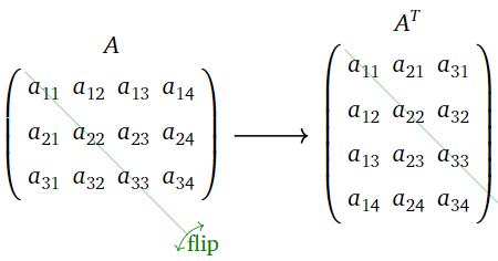
Figure \(\PageIndex{3}\)
Like inversion, transposition reverses the order of matrix multiplication.
Let \(A\) be an \(m\times n\) matrix, and let \(B\) be an \(n\times p\) matrix. Then
\[ (AB)^T = B^TA^T. \nonumber \]
- Proof
-
First suppose that \(A\) is a row vector an \(B\) is a column vector, i.e., \(m = p = 1\). Then
\[\begin{aligned}AB&=\left(\begin{array}{cccc}a_1 &a_2&\cdots &a_n\end{array}\right)\left(\begin{array}{c}b_1\\b_2\\ \vdots\\b_n\end{array}\right)=a_1b_1+a_2b_2+\cdots +a_nb_n \\ &=\left(\begin{array}{cccc}b_1&b_2&\cdots &b_n\end{array}\right)\left(\begin{array}{c}a_1\\a_2\\ \vdots\\a_n\end{array}\right)=B^TA^T.\end{aligned}\]
Now we use the row-column rule for matrix multiplication. Let \(r_1,r_2,\ldots,r_m\) be the rows of \(A\text{,}\) and let \(c_1,c_2,\ldots,c_p\) be the columns of \(B\text{,}\) so
\[AB=\left(\begin{array}{c}—r_1 —\\ —r_2— \\ \vdots \\ —r_m—\end{array}\right)\left(\begin{array}{cccc}|&|&\quad &| \\ c_1&c_2&\cdots &c_p \\ |&|&\quad &|\end{array}\right)=\left(\begin{array}{cccc}r_1c_1&r_1c_2&\cdots &r_1c_p \\ r_2c_1&r_2c_2&\cdots &r_2c_p \\ \vdots &\vdots &{}&\vdots \\ r_mc_1&r_mc_2&\cdots &r_mc_p\end{array}\right).\nonumber\]
By the case we handled above, we have \(r_ic_j = c_j^Tr_i^T\). Then
\[\begin{aligned}(AB)^T&=\left(\begin{array}{cccc}r_1c_1&r_2c_1&\cdots &r_mc_1 \\ r_1c_2&r_2c_2&\cdots &r_mc_2 \\ \vdots &\vdots &{}&\vdots \\ r_1c_p&r_2c_p&\cdots &r_mc_p\end{array}\right) \\ &=\left(\begin{array}{cccc}c_1^Tr_1^T &c_1^Tr_2^T&\cdots &c_1^Tr_m^T \\ c_2^Tr_1^T&c_2^Tr_2^T&\cdots &c_2^Tr_m^T \\ \vdots&\vdots&{}&\vdots \\ c_p^Tr_1^T&c_p^Tr_2^T&\cdots&c_p^Tr_m^T\end{array}\right) \\ &=\left(\begin{array}{c}—c_1^T— \\ —c_2^T— \\ \vdots \\ —c_p^T—\end{array}\right)\left(\begin{array}{cccc}|&|&\quad&| \\ r_1^T&r_2^T&\cdots&r_m^T \\ |&|&\quad&|\end{array}\right)=B^TA^T.\end{aligned}\]
For any square matrix \(A\text{,}\) we have
\[ \det(A) = \det(A^T). \nonumber \]
- Proof
-
We follow the same strategy as in the proof of the multiplicativity property, Proposition \(\PageIndex{3}\): namely, we define
\[ d(A) = \det(A^T), \nonumber \]
and we show that \(d\) satisfies the four defining properties of the determinant. Again we use elementary matrices, also introduced in the proof of the multiplicativity property, Proposition \(\PageIndex{3}\).
- Let \(C'\) be the matrix obtained by doing a row replacement on \(C\text{,}\) and let \(E\) be the elementary matrix for this row replacement, so \(C' = EC\). The elementary matrix for a row replacement is either upper-triangular or lower-triangular, with ones on the diagonal: \[R_1=R_1+3R_3:\left(\begin{array}{ccc}1&0&3\\0&1&0\\0&0&1\end{array}\right)\quad R_3=R_3+3R_1:\left(\begin{array}{ccc}1&0&0\\0&1&0\\3&0&1\end{array}\right).\nonumber\]
It follows that \(E^T\) is also either upper-triangular or lower-triangular, with ones on the diagonal, so \(\det(E^T) = 1\) by this Proposition \(\PageIndex{1}\). By the Fact \(\PageIndex{1}\) and the multiplicativity property, Proposition \(\PageIndex{3}\), \[ \begin{split} d(C') \amp= \det((C')^T) = \det((EC)^T) = \det(C^TE^T) \\ \amp= \det(C^T)\det(E^T) = \det(C^T) = d(C). \end{split} \nonumber \] - Let \(C'\) be the matrix obtained by scaling a row of \(C\) by a factor of \(c\text{,}\) and let \(E\) be the elementary matrix for this row replacement, so \(C' = EC\). Then \(E\) is a diagonal matrix: \[R_2=cR_2:\: \left(\begin{array}{ccc}1&0&0\\0&c&0\\0&0&1\end{array}\right).\nonumber\] Thus \(\det(E^T) = c\). By the Fact \(\PageIndex{1}\) and the multiplicativity property, Proposition \(\PageIndex{3}\), \[ \begin{split} d(C') \amp= \det((C')^T) = \det((EC)^T) = \det(C^TE^T) \\ \amp= \det(C^T)\det(E^T) = c\det(C^T) = c\cdot d(C). \end{split} \nonumber \]
- Let \(C'\) be the matrix obtained by swapping two rows of \(C\text{,}\) and let \(E\) be the elementary matrix for this row replacement, so \(C' = EC\). The \(E\) is equal to its own transpose: \[R_1\longleftrightarrow R_2:\:\left(\begin{array}{ccc}0&1&0\\1&0&0\\0&0&1\end{array}\right)=\left(\begin{array}{ccc}0&1&0\\1&0&0\\0&0&1\end{array}\right)^T.\nonumber\] Since \(E\) (hence \(E^T\)) is obtained by performing one row swap on the identity matrix, we have \(\det(E^T) = -1\). By the Fact \(\PageIndex{1}\) and the multiplicativity property, Proposition \(\PageIndex{3}\), \[ \begin{split} d(C') \amp= \det((C')^T) = \det((EC)^T) = \det(C^TE^T) \\ \amp= \det(C^T)\det(E^T) = -\det(C^T) = - d(C). \end{split} \nonumber \]
- Since \(I_n^T = I_n,\) we have \[ d(I_n) = \det(I_n^T) = det(I_n) = 1. \nonumber \] Since \(d\) satisfies the four defining properties of the determinant, it is equal to the determinant by the existence theorem \(\PageIndex{1}\). In other words, for all matrices \(A\text{,}\) we have\[ \det(A) = d(A) = \det(A^T). \nonumber \]
- Let \(C'\) be the matrix obtained by doing a row replacement on \(C\text{,}\) and let \(E\) be the elementary matrix for this row replacement, so \(C' = EC\). The elementary matrix for a row replacement is either upper-triangular or lower-triangular, with ones on the diagonal: \[R_1=R_1+3R_3:\left(\begin{array}{ccc}1&0&3\\0&1&0\\0&0&1\end{array}\right)\quad R_3=R_3+3R_1:\left(\begin{array}{ccc}1&0&0\\0&1&0\\3&0&1\end{array}\right).\nonumber\]
The transpose property, Proposition \(\PageIndex{4}\), is very useful. For concreteness, we note that \(\det(A)=\det(A^T)\) means, for instance, that
\[ \det\left(\begin{array}{ccc}1&2&3\\4&5&6\\7&8&9\end{array}\right) = \det\left(\begin{array}{ccc}1&4&7\\2&5&8\\3&6&9\end{array}\right). \nonumber \]
This implies that the determinant has the curious feature that it also behaves well with respect to column operations. Indeed, a column operation on \(A\) is the same as a row operation on \(A^T\text{,}\) and \(\det(A) = \det(A^T)\).
The determinant satisfies the following properties with respect to column operations:
- Doing a column replacement on \(A\) does not change \(\det(A)\).
- Scaling a column of \(A\) by a scalar \(c\) multiplies the determinant by \(c\).
- Swapping two columns of a matrix multiplies the determinant by \(-1\).
The previous corollary makes it easier to compute the determinant: one is allowed to do row and column operations when simplifying the matrix. (Of course, one still has to keep track of how the row and column operations change the determinant.)
Compute \(\det\left(\begin{array}{ccc}2&7&4\\3&1&3\\4&0&1\end{array}\right).\)
Solution
It takes fewer column operations than row operations to make this matrix upper-triangular:
\[\begin{aligned}\left(\begin{array}{ccc}2&7&4\\3&1&3\\4&0&1\end{array}\right)\quad\xrightarrow{C_1=C_1-4C_3}\quad &\left(\begin{array}{ccc}-14&7&4\\-9&1&3\\0&0&1\end{array}\right) \\ {}\xrightarrow{C_1=C_1+9C_2}\quad&\left(\begin{array}{ccc}49&7&4\\0&1&3\\0&0&1\end{array}\right)\end{aligned}\]
We performed two column replacements, which does not change the determinant; therefore,
\[ \det\left(\begin{array}{ccc}2&7&4\\3&1&3\\4&0&1\end{array}\right) = \det\left(\begin{array}{ccc}49&7&4\\0&1&3\\0&0&1\end{array}\right) = 49. \nonumber \]
Multilinearity
The following observation is useful for theoretical purposes.
We can think of \(\det\) as a function of the rows of a matrix:
\[ \det(v_1,v_2,\ldots,v_n) = \det\left(\begin{array}{c}—v_1— \\ —v_2— \\ \vdots \\ —v_n—\end{array}\right). \nonumber \]
Let \(i\) be a whole number between \(1\) and \(n\text{,}\) and fix \(n-1\) vectors \(v_1,v_2,\ldots,v_{i-1},v_{i+1},\ldots,v_n\) in \(\mathbb{R}^n \). Then the transformation \(T\colon\mathbb{R}^n \to\mathbb{R}\) defined by
\[ T(x) = \det(v_1,v_2,\ldots,v_{i-1},x,v_{i+1},\ldots,v_n) \nonumber \]
is linear.
- Proof
-
First assume that \(i=1\text{,}\) so
\[ T(x) = \det(x,v_2,\ldots,v_n). \nonumber \]
We have to show that \(T\) satisfies the defining properties, Definition 3.3.1, in Section 3.3.
- By the first defining property, Definition \(\PageIndex{1}\), scaling any row of a matrix by a number \(c\) scales the determinant by a factor of \(c\). This implies that \(T\) satisfies the second property, i.e., that \[ T(cx) = \det(cx,v_2,\ldots,v_n) = c\det(x,v_2,\ldots,v_n) = cT(x). \nonumber \]
- We claim that \(T(v+w) = T(v) + T(w)\). If \(w\) is in \(\text{Span}\{v,v_2,\ldots,v_n\}\text{,}\) then \[ w = cv + c_2v_2 + \cdots + c_nv_n \nonumber \] for some scalars \(c,c_2,\ldots,c_n\). Let \(A\) be the matrix with rows \(v+w,v_2,\ldots,v_n\text{,}\) so \(T(v+w) = \det(A).\) By performing the row operations \[ R_1 = R_1 - c_2R_2;\quad R_1 = R_1 - c_3R_3;\quad\ldots\quad R_1 = R_1 - c_nR_n, \nonumber \] the first row of the matrix \(A\) becomes \[ v+w-(c_2v_2+\cdots+c_nv_n) = v + cv = (1+c)v. \nonumber \] Therefore, \[ \begin{split} T(v+w) = \det(A) \amp= \det((1+c)v,v_2,\ldots,v_n) \\ \amp= (1+c)\det(v,v_2,\ldots,v_n) \\ \amp= T(v) + cT(v) = T(v) + T(cv). \end{split} \nonumber \] Doing the opposite row operations \[ R_1 = R_1 + c_2R_2;\quad R_1 = R_1 + c_3R_3;\quad\ldots\quad R_1 = R_1 + c_nR_n \nonumber \] to the matrix with rows \(cv,v_2,\ldots,v_n\) shows that \[ \begin{split} T(cv) \amp= \det(cv,v_2,\ldots,v_n) \\ \amp= \det(cv+c_2v_2+\cdots+c_nv_n,v_2,\ldots,v_n) \\ \amp= \det(w,v_2,\ldots,v_n) = T(w), \end{split} \nonumber \] which finishes the proof of the first property in this case.
Now suppose that \(w\) is not in \(\text{Span}\{v,v_2,\ldots,v_n\}\). This implies that \(\{v,v_2,\ldots,v_n\}\) is linearly dependent (otherwise it would form a basis for \(\mathbb{R}^n \)), so \(T(v)\) = 0. If \(v\) is not in \(\text{Span}\{v_2,\ldots,v_n\}\text{,}\) then \(\{v_2,\ldots,v_n\}\) is linearly dependent by the increasing span criterion, Theorem 2.5.2 in Section 2.5, so \(T(x) = 0\) for all \(x\text{,}\) as the matrix with rows \(x,v_2,\ldots,v_n\) is not invertible. Hence we may assume \(v\) is in \(\text{Span}\{v_2,\ldots,v_n\}\). By the above argument with the roles of \(v\) and \(w\) reversed, we have \(T(v+w) = T(v)+T(w).\)
For \(i\neq 1\text{,}\) we note that
\[ \begin{split} T(x) \amp= \det(v_1,v_2,\ldots,v_{i-1},x,v_{i+1},\ldots,v_n) \\ \amp= -\det(x,v_2,\ldots,v_{i-1},v_1,v_{i+1},\ldots,v_n). \end{split} \nonumber \]
By the previously handled case, we know that \(-T\) is linear:
\[ -T(cx) = -cT(x) \qquad -T(v+w) = -T(v) - T(w). \nonumber \]
Multiplying both sides by \(-1\text{,}\) we see that \(T\) is linear.
For example, we have
\[\det\left(\begin{array}{lcr}—&v_1&— \\ —&av+bw&— \\ —&v_3&—\end{array}\right)=a\det\left(\begin{array}{c}—v_1— \\ —v— \\ —v_3—\end{array}\right)+b\det\left(\begin{array}{c}—v_1— \\ —w— \\ —v_3—\end{array}\right)\nonumber\]
By the transpose property, Proposition \(\PageIndex{4}\), the determinant is also multilinear in the columns of a matrix:
\[ \det\left(\begin{array}{ccc}|&|&|\\ v_1&av+bw&v_3 \\ |&|&|\end{array}\right) = a\det\left(\begin{array}{ccc}|&|&|\\v_1&v&v_3 \\ |&|&|\end{array}\right) + b\det\left(\begin{array}{ccc}|&|&|\\v_1&w&v_3\\|&|&|\end{array}\right). \nonumber \]
In more theoretical treatments of the topic, where row reduction plays a secondary role, the defining properties of the determinant are often taken to be:
- The determinant \(\det(A)\) is multilinear in the rows of \(A\).
- If \(A\) has two identical rows, then \(\det(A) = 0\).
- The determinant of the identity matrix is equal to one.
We have already shown that our four defining properties, Definition \(\PageIndex{1}\), imply these three. Conversely, we will prove that these three alternative properties imply our four, so that both sets of properties are equivalent.
Defining property \(2\) is just the second defining property, Definition 3.3.1, in Section 3.3. Suppose that the rows of \(A\) are \(v_1,v_2,\ldots,v_n\). If we perform the row replacement \(R_i = R_i + cR_j\) on \(A\text{,}\) then the rows of our new matrix are \(v_1,v_2,\ldots,v_{i-1},v_i+cv_j,v_{i+1},\ldots,v_n\text{,}\) so by linearity in the \(i\)th row,
\[ \begin{split} \det(\amp v_1,v_2,\ldots,v_{i-1},v_i+cv_j,v_{i+1},\ldots,v_n) \\ \amp= \det(v_1,v_2,\ldots,v_{i-1},v_i,v_{i+1},\ldots,v_n) + c\det(v_1,v_2,\ldots,v_{i-1},v_j,v_{i+1},\ldots,v_n) \\ \amp= \det(v_1,v_2,\ldots,v_{i-1},v_i,v_{i+1},\ldots,v_n) = \det(A), \end{split} \nonumber \]
where \(\det(v_1,v_2,\ldots,v_{i-1},v_j,v_{i+1},\ldots,v_n)=0\) because \(v_j\) is repeated. Thus, the alternative defining properties imply our first two defining properties. For the third, suppose that we want to swap row \(i\) with row \(j\). Using the second alternative defining property and multilinearity in the \(i\)th and \(j\)th rows, we have
\[ \begin{split} 0 \amp= \det(v_1,\ldots,v_i+v_j,\ldots,v_i+v_j,\ldots,v_n) \\ \amp= \det(v_1,\ldots,v_i,\ldots,v_i+v_j,\ldots,v_n) + \det(v_1,\ldots,v_j,\ldots,v_i+v_j,\ldots,v_n) \\ \amp= \det(v_1,\ldots,v_i,\ldots,v_i,\ldots,v_n) + \det(v_1,\ldots,v_i,\ldots,v_j,\ldots,v_n) \\ \amp\qquad+\det(v_1,\ldots,v_j,\ldots,v_i,\ldots,v_n) + \det(v_1,\ldots,v_j,\ldots,v_j,\ldots,v_n) \\ \amp= \det(v_1,\ldots,v_i,\ldots,v_j,\ldots,v_n) + \det(v_1,\ldots,v_j,\ldots,v_i,\ldots,v_n), \end{split} \nonumber \]
as desired.
We have
\[ \left(\begin{array}{c}-1\\2\\3\end{array}\right) = -\left(\begin{array}{c}1\\0\\0\end{array}\right) + 2\left(\begin{array}{c}0\\1\\0\end{array}\right) + 3\left(\begin{array}{c}0\\0\\1\end{array}\right). \nonumber \]
Therefore,
\[ \begin{split} \det\amp\left(\begin{array}{ccc}-1&7&2\\2&-3&2\\3&1&1\end{array}\right) = -\det\left(\begin{array}{ccc}1&7&2\\0&-3&2\\0&1&1\end{array}\right) \\ \amp+ 2\det\left(\begin{array}{ccc}0&7&2\\1&-3&2\\0&1&1\end{array}\right) + 3\det\left(\begin{array}{ccc}0&7&2\\0&-3&2\\1&1&1\end{array}\right). \end{split} \nonumber \]
This is the basic idea behind cofactor expansions in Section 4.2.
- There is one and only one function \(\det\colon\{n\times n\text{ matrices}\}\to\mathbb{R}\) satisfying the four defining properties, Definition \(\PageIndex{1}\).
- The determinant of an upper-triangular or lower-triangular matrix is the product of the diagonal entries.
- A square matrix is invertible if and only if \(\det(A)\neq 0\text{;}\) in this case, \[ \det(A^{-1}) = \frac 1{\det(A)}. \nonumber \]
- If \(A\) and \(B\) are \(n\times n\) matrices, then \[ \det(AB) = \det(A)\det(B). \nonumber \]
- For any square matrix \(A\text{,}\) we have \[ \det(A^T) = \det(A). \nonumber \]
- The determinant can be computed by performing row and/or column operations.