6.3: Orthogonal Projection

$\usepackage{macros} \newcommand{\lt}{<} \newcommand{\gt}{>} \newcommand{\amp}{&}$

Learning Objectives

1. Understand the orthogonal decomposition of a vector with respect to a subspace.
2. Understand the relationship between orthogonal decomposition and orthogonal projection.
3. Understand the relationship between orthogonal decomposition and the closest vector on / distance to a subspace.
4. Learn the basic properties of orthogonal projections as linear transformations and as matrix transformations.
5. Recipes: orthogonal projection onto a line, orthogonal decomposition by solving a system of equations, orthogonal projection via a complicated matrix product.
6. Pictures: orthogonal decomposition, orthogonal projection.
7. Vocabulary words: orthogonal decomposition, orthogonal projection.

Let $W$ be a subspace of $\mathbb{R}^n$ and let $x$ be a vector in $\mathbb{R}^n$. In this section, we will learn to compute the closest vector $x_W$ to $x$ in $W$. The vector $x_W$ is called the orthogonal projection of $x$ onto $W$. This is exactly what we will use to almost solve matrix equations, as discussed in the introduction to Chapter 6.

Orthogonal Decomposition

We begin by fixing some notation.

Definition $\PageIndex{1}$: Notation

Let $W$ be a subspace of $\mathbb{R}^n$ and let $x$ be a vector in $\mathbb{R}^n$. We denote the closest vector to $x$ on $W$ by $x_W$.

To say that $x_W$ is the closest vector to $x$ on $W$ means that the difference $x-x_W$ is orthogonal to the vectors in $W\text{:}$

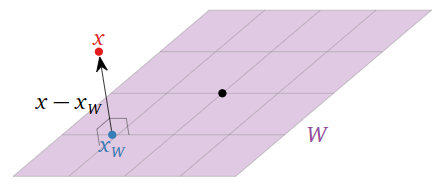
Figure $\PageIndex{1}$

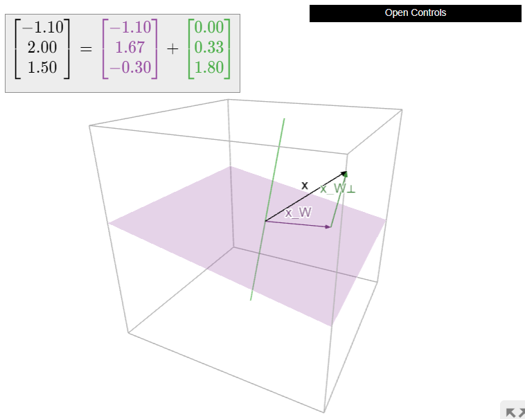
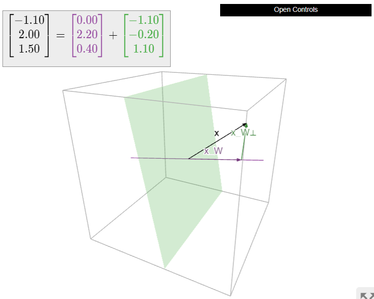
In other words, if $x_{W^\perp} = x - x_W\text{,}$ then we have $x = x_W + x_{W^\perp}\text{,}$ where $x_W$ is in $W$ and $x_{W^\perp}$ is in $W^\perp$. The first order of business is to prove that the closest vector always exists.

Theorem $\PageIndex{1}$: Orthogonal Decomposition

Let $W$ be a subspace of $\mathbb{R}^n$ and let $x$ be a vector in $\mathbb{R}^n$. Then we can write $x$ uniquely as

$$x = x_W + x_{W^\perp} \nonumber$$

where $x_W$ is the closest vector to $x$ on $W$ and $x_{W^\perp}$ is in $W^\perp$.

Proof

Let $m = \dim(W)\text{,}$ so $n-m = \dim(W^\perp)$ by Fact 6.2.1 in Section 6.2. Let $v_1,v_2,\ldots,v_m$ be a basis for $W$ and let $v_{m+1},v_{m+2},\ldots,v_n$ be a basis for $W^\perp$. We showed in the proof of this Fact 6.2.1 in Section 6.2 that $\{v_1,v_2,\ldots,v_m,v_{m+1},v_{m+2},\ldots,v_n\}$ is linearly independent, so it forms a basis for $\mathbb{R}^n$. Therefore, we can write

$$x = (c_1v_1 + \cdots + c_mv_m) + (c_{m+1}v_{m+1} + \cdots + c_nv_n) = x_W + x_{W^\perp}, \nonumber$$

where $x_W = c_1v_1 + \cdots + c_mv_m$ and $x_{W^\perp} = c_{m+1}v_{m+1} + \cdots + c_nv_n$. Since $x_{W^\perp}$ is orthogonal to $W\text{,}$ the vector $x_W$ is the closest vector to $x$ on $W\text{,}$ so this proves that such a decomposition exists.

As for uniqueness, suppose that

$$x = x_W + x_{W^\perp} = y_W + y_{W^\perp} \nonumber$$

for $x_W,y_W$ in $W$ and $x_{W^\perp},y_{W^\perp}$ in $W^\perp$. Rearranging gives

$$x_W - y_W = y_{W^\perp} - x_{W^\perp}. \nonumber$$

Since $W$ and $W^\perp$ are subspaces, the left side of the equation is in $W$ and the right side is in $W^\perp$. Therefore, $x_W-y_W$ is in $W$ and in $W^\perp\text{,}$ so it is orthogonal to itself, which implies $x_W-y_W=0$. Hence $x_W = y_W$ and $x_{W^\perp} = y_{W^\perp}\text{,}$ which proves uniqueness.

Definition $\PageIndex{2}$: Orthogonal Decomposition and Orthogonal Projection

Let $W$ be a subspace of $\mathbb{R}^n$ and let $x$ be a vector in $\mathbb{R}^n$. The expression

$$x = x_W + x_{W^\perp} \nonumber$$

for $x_W$ in $W$ and $x_{W^\perp}$ in $W^\perp\text{,}$ is called the orthogonal decomposition of $x$ with respect to $W\text{,}$ and the closest vector $x_W$ is the orthogonal projection of $x$ onto $W$.

Since $x_W$ is the closest vector on $W$ to $x\text{,}$ the distance from $x$ to the subspace $W$ is the length of the vector from $x_W$ to $x\text{,}$ i.e., the length of $x_{W^\perp}$. To restate:

Note $\PageIndex{1}$: Closest Vector and Distance

Let $W$ be a subspace of $\mathbb{R}^n$ and let $x$ be a vector in $\mathbb{R}^n$.

• The orthogonal projection $x_W$ is the closest vector to $x$ in $W$.
• The distance from $x$ to $W$ is $\|x_{W^\perp}\|$.

Example $\PageIndex{1}$: Orthogonal decomposition with respect to the $xy$-plane

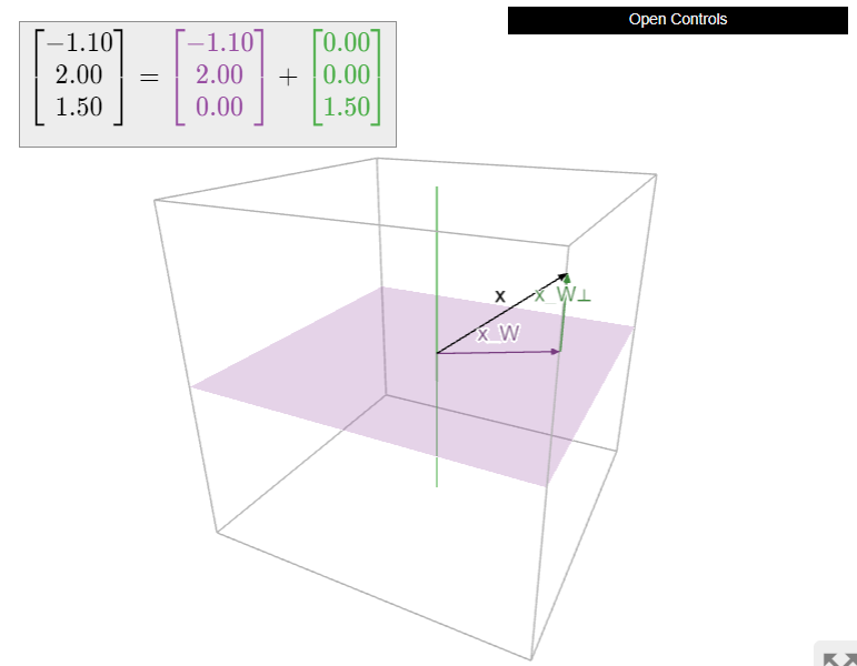
Let $W$ be the $xy$-plane in $\mathbb{R}^3 \text{,}$ so $W^\perp$ is the $z$-axis. It is easy to compute the orthogonal decomposition of a vector with respect to this $W\text{:}$

$$\begin{aligned}x&=\left(\begin{array}{c}1\\2\\3\end{array}\right)\implies x_W=\left(\begin{array}{c}1\\2\\0\end{array}\right)\:\:x_{W^{\perp}}=\left(\begin{array}{c}0\\0\\3\end{array}\right) \\ x&=\left(\begin{array}{c}a\\b\\c\end{array}\right)\implies x_W=\left(\begin{array}{c}a\\b\\0\end{array}\right)\:\:x_{W^{\perp}}=\left(\begin{array}{c}0\\0\\c\end{array}\right).\end{aligned}$$

We see that the orthogonal decomposition in this case expresses a vector in terms of a “horizontal” component (in the $xy$-plane) and a “vertical” component (on the $z$-axis).

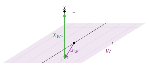
Figure $\PageIndex{2}$

Figure $\PageIndex{3}$: Orthogonal decomposition of a vector with respect to the $xy$-plane in $\mathbb{R}^3$. Note that $\color{Purple}x_W$ is in the $xy$-plane and $\color{Green}x_{W^\perp}$ is in the $z$-axis. Click and drag the head of the vector $x$ to see how the orthogonal decomposition changes.

Example $\PageIndex{2}$: Orthogonal decomposition of a vector in $W$

If $x$ is in a subspace $W\text{,}$ then the closest vector to $x$ in $W$ is itself, so $x = x_W$ and $x_{W^\perp} = 0$. Conversely, if $x = x_W$ then $x$ is contained in $W$ because $x_W$ is contained in $W$.

Example $\PageIndex{3}$: Orthogonal decomposition of a vector in $W^\perp$

If $W$ is a subspace and $x$ is in $W^\perp\text{,}$ then the orthogonal decomposition of $x$ is $x = 0 + x\text{,}$ where $0$ is in $W$ and $x$ is in $W^\perp$. It follows that $x_W = 0$. Conversely, if $x_W = 0$ then the orthogonal decomposition of $x$ is $x = x_W + x_{W^\perp} = 0 + x_{W^\perp}\text{,}$ so $x = x_{W^\perp}$ is in $W^\perp$.

Example $\PageIndex{4}$: Interactive: Orthogonal decomposition in $\mathbb{R}^2$

Figure $\PageIndex{4}$: Orthogonal decomposition of a vector with respect to a line $W$ in $\mathbb{R}^2$. Note that $\color{Purple}x_W$ is in $W$ and $\color{Green}x_{W^\perp}$ is in the line perpendicular to $W$. Click and drag the head of the vector $x$ to see how the orthogonal decomposition changes.

Example $\PageIndex{5}$: Interactive: Orthogonal decomposition in $\mathbb{R}^3$

Figure $\PageIndex{5}$: Orthogonal decomposition of a vector with respect to a plane $W$ in $\mathbb{R}^3$. Note that $\color{Purple}x_W$ is in $W$ and $\color{Green}x_{W^\perp}$ is in the line perpendicular to $W$. Click and drag the head of the vector $x$ to see how the orthogonal decomposition changes.

Example $\PageIndex{6}$: Interactive: Orthogonal decomposition in $\mathbb{R}^3$

Figure $\PageIndex{6}$: Orthogonal decomposition of a vector with respect to a line $W$ in $\mathbb{R}^3$. Note that $\color{Purple}x_W$ is in $W$ and $\color{Green}x_{W^\perp}$ is in the plane perpendicular to $W$. Click and drag the head of the vector $x$ to see how the orthogonal decomposition changes.

Now we turn to the problem of computing $x_W$ and $x_{W^\perp}$. Of course, since $x_{W^\perp} = x - x_W\text{,}$ really all we need is to compute $x_W$. The following theorem gives a method for computing the orthogonal projection onto a column space. To compute the orthogonal projection onto a general subspace, usually it is best to rewrite the subspace as the column space of a matrix, as in Note 2.6.3 in Section 2.6.

Theorem$\PageIndex{2}$

Let $A$ be an $m \times n$ matrix, let $W = \text{Col}(A)\text{,}$ and let $x$ be a vector in $\mathbb{R}^m$. Then the matrix equation

$$A^TAc=A^Tx \nonumber$$

in the unknown vector $c$ is consistent, and $x_W$ is equal to $Ac$ for any solution $c$.

Proof

Let $x = x_W + x_{W^\perp}$ be the orthogonal decomposition with respect to $W$. By definition $x_W$ lies in $W=\text{Col}(A)$ and so there is a vector $c$ in $\mathbb{R}^n$ with $Ac = x_W$. Choose any such vector $c$. We know that $x-x_W=x-Ac$ lies in $W^\perp\text{,}$ which is equal to $\text{Nul}(A^T)$ by Recipe: Shortcuts for Computing Orthogonal Complements in Section 6.2. We thus have

$$0=A^T(x-Ac) = A^Tx-A^TAc \nonumber$$

and so

$$A^TAc = A^Tx. \nonumber$$

This exactly means that $A^TAc = A^Tx$ is consistent. If $c$ is any solution to $A^TAc=A^Tx$ then by reversing the above logic, we conclude that $x_W = Ac$.

Example $\PageIndex{7}$: Orthogonal Projection onto a Line

Let $L = \text{Span}\{u\}$ be a line in $\mathbb{R}^n$ and let $x$ be a vector in $\mathbb{R}^n$. By Theorem $\PageIndex{2}$, to find $x_L$ we must solve the matrix equation $u^Tuc = u^Tx\text{,}$ where we regard $u$ as an $n\times 1$ matrix (the column space of this matrix is exactly $L\text{!}$). But $u^Tu = u\cdot u$ and $u^Tx = u\cdot x\text{,}$ so $c = (u\cdot x)/(u\cdot u)$ is a solution of $u^Tuc = u^Tx\text{,}$ and hence $x_L = uc = (u\cdot x)/(u\cdot u)\,u.$

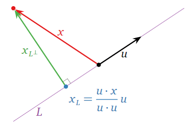
Figure $\PageIndex{7}$

To reiterate:

Recipe: Orthogonal Projection onto a Line

If $L = \text{Span}\{u\}$ is a line, then

$$x_L = \frac{u\cdot x}{u\cdot u}\,u \quad\text{and}\quad x_{L^\perp} = x - x_L \nonumber$$

for any vector $x$.

Remark: Simple proof for the formula for projection onto a line

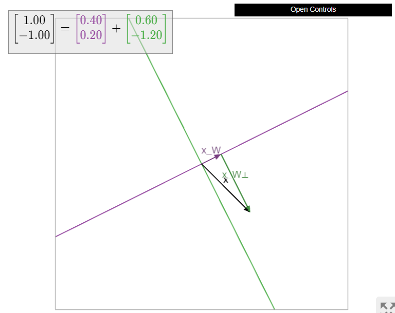
In the special case where we are projecting a vector $x$ in $\mathbb{R}^n$ onto a line $L = \text{Span}\{u\}\text{,}$ our formula for the projection can be derived very directly and simply. The vector $x_L$ is a multiple of $u\text{,}$ say $x_L=cu$. This multiple is chosen so that $x-x_L=x-cu$ is perpendicular to $u\text{,}$ as in the following picture.

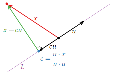
Figure $\PageIndex{8}$

In other words,

$$(x-cu) \cdot u = 0. \nonumber$$

Using the distributive property for the dot product and isolating the variable $c$ gives us that

$$c = \frac{u\cdot x}{u\cdot u} \nonumber$$

and so

$$x_L = cu = \frac{u\cdot x}{u\cdot u}\,u. \nonumber$$

Example $\PageIndex{8}$: Projection onto a line in $\mathbb{R}^2$

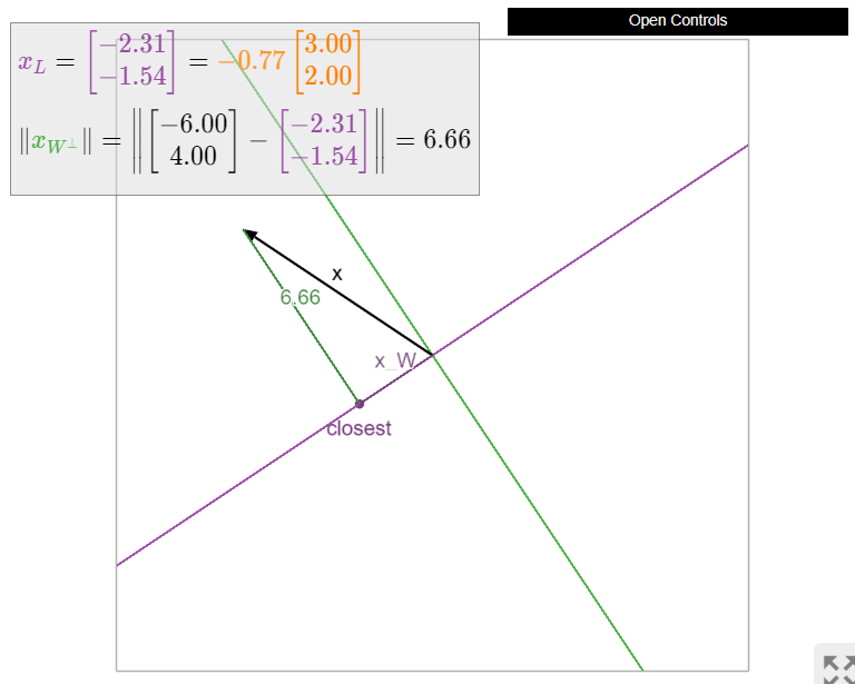
Compute the orthogonal projection of $x = {-6\choose 4}$ onto the line $L$ spanned by $u = {3\choose 2}\text{,}$ and find the distance from $x$ to $L$.

Solution

First we find

$$x_L = \frac{x\cdot u}{u\cdot u}\,u = \frac{-18+8}{9+4}\left(\begin{array}{c}3\\2\end{array}\right) = -\frac{10}{13}\left(\begin{array}{c}3\\2\end{array}\right) \qquad x_{L^\perp} = x - x_L = \frac 1{13}\left(\begin{array}{c}-48\\72\end{array}\right). \nonumber$$

The distance from $x$ to $L$ is

$$\|x_{L^\perp}\| = \frac 1{13}\sqrt{48^2 + 72^2} \approx 6.656. \nonumber$$

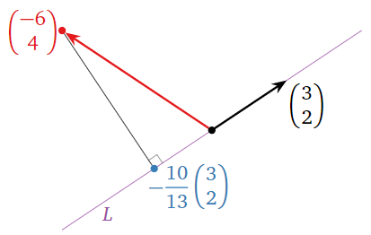
Figure $\PageIndex{9}$

Figure $\PageIndex{10}$: Distance from the line $L$.

Example $\PageIndex{9}$: Projection onto a line in $\mathbb{R}^3$

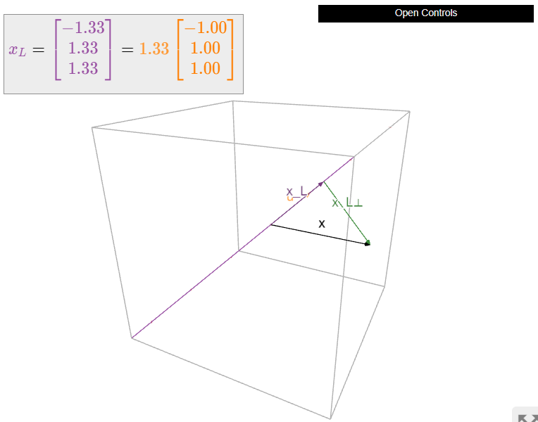
Let

$$x = \left(\begin{array}{c}-2\\3\\-1\end{array}\right) \qquad u = \left(\begin{array}{c}-1\\1\\1\end{array}\right), \nonumber$$

and let $L$ be the line spanned by $u$. Compute $x_L$ and $x_L^\perp$.

Solution

$$x_L = \frac{x\cdot u}{u\cdot u}\,u = \frac{2+3-1}{1+1+1}\left(\begin{array}{c}-1\\1\\1\end{array}\right) = \frac{4}{3}\left(\begin{array}{c}-1\\1\\1\end{array}\right) \qquad x_{L^\perp} = x - x_L = \frac 13\left(\begin{array}{c}-2\\5\\-7\end{array}\right). \nonumber$$

Figure $\PageIndex{11}$: Orthogonal projection onto the line $L$.

When $A$ is a matrix with more than one column, computing the orthogonal projection of $x$ onto $W = \text{Col}(A)$ means solving the matrix equation $A^TAc = A^Tx$. In other words, we can compute the closest vector by solving a system of linear equations. To be explicit, we state Theorem $\PageIndex{2}$ as a recipe:

Recipe: Compute an Orthogonal Decomposition

Let $W$ be a subspace of $\mathbb{R}^m$. Here is a method to compute the orthogonal decomposition of a vector $x$ with respect to $W\text{:}$

0. Rewrite $W$ as the column space of a matrix $A$. In other words, find a a spanning set for $W\text{,}$ and let $A$ be the matrix with those columns.
1. Compute the matrix $A^TA$ and the vector $A^Tx$.
2. Form the augmented matrix for the matrix equation $A^TAc = A^Tx$ in the unknown vector $c\text{,}$ and row reduce.
3. This equation is always consistent; choose one solution $c$. Then $$x_W = Ac \qquad x_{W^\perp} = x - x_W. \nonumber$$

Example $\PageIndex{10}$: Projection onto the $xy$-plane

Use Theorem $\PageIndex{2}$ to compute the orthogonal decomposition of a vector with respect to the $xy$-plane in $\mathbb{R}^3$.

Solution

A basis for the $xy$-plane is given by the two standard coordinate vectors

$$e_1 = \left(\begin{array}{c}1\\0\\0\end{array}\right) \qquad e_2 =\left(\begin{array}{c}0\\1\\0\end{array}\right). \nonumber$$

Let $A$ be the matrix with columns $e_1,e_2\text{:}$

$$A = \left(\begin{array}{cc}1&0\\0&1\\0&0\end{array}\right). \nonumber$$

Then

$$A^TA = \left(\begin{array}{cc}1&0\\0&1\end{array}\right) = I_2 \qquad A^T\left(\begin{array}{c}x_1\\x_2\\x_3\end{array}\right) = \left(\begin{array}{ccc}1&0&0\\0&1&0\end{array}\right)\left(\begin{array}{c}x_1\\x_2\\x_3\end{array}\right) = \left(\begin{array}{c}x_1\\x_2\end{array}\right). \nonumber$$

It follows that the unique solution $c$ of $A^TAc = I_2c = A^Tx$ is given by the first two coordinates of $x\text{,}$ so

$$x_W = A\left(\begin{array}{c}x_1\\x_2\end{array}\right) = \left(\begin{array}{cc}1&0\\0&1\\0&0\end{array}\right)\left(\begin{array}{c}x_1\\x_2\end{array}\right) = \left(\begin{array}{c}x_1\\x_2\\0\end{array}\right) \qquad x_{W^\perp} = x - x_W = \left(\begin{array}{c}0\\0\\x_3\end{array}\right). \nonumber$$

We have recovered this Example $\PageIndex{1}$.

Example $\PageIndex{11}$: Projection onto a plane in $\mathbb{R}^3$

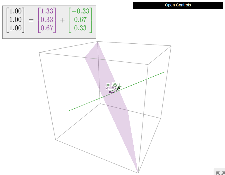
Let

$$W = \text{Span}\left\{\left(\begin{array}{c}1\\0\\-1\end{array}\right),\;\left(\begin{array}{c}1\\1\\0\end{array}\right)\right\} \qquad x = \left(\begin{array}{c}1\\2\\3\end{array}\right). \nonumber$$

Compute $x_W$ and the distance from $x$ to $W$.

Solution

We have to solve the matrix equation $A^TAc = A^Tx\text{,}$ where

$$A = \left(\begin{array}{cc}1&1\\0&1\\-1&0\end{array}\right). \nonumber$$

We have

$$A^TA = \left(\begin{array}{cc}2&1\\1&2\end{array}\right) \qquad A^Tx = \left(\begin{array}{c}-2\\3\end{array}\right). \nonumber$$

We form an augmented matrix and row reduce:

$$\left(\begin{array}{cc|c}2&1&-2\\1&2&3\end{array}\right)\xrightarrow{\text{RREF}}\left(\begin{array}{cc|c} 1&0&-7/3 \\ 0&1&8/3\end{array}\right) \implies c = \frac 13\left(\begin{array}{c}-7\\8\end{array}\right). \nonumber$$

It follows that

$$x_W = Ac = \frac 13\left(\begin{array}{c}1\\8\\7\end{array}\right) \qquad x_{W^\perp} = x - x_W = \frac 13\left(\begin{array}{c}2\\-2\\2\end{array}\right). \nonumber$$

The distance from $x$ to $W$ is

$$\|x_{W^\perp}\| = \frac 1{3}\sqrt{4+4+4} \approx 1.155. \nonumber$$

Figure $\PageIndex{12}$: Orthogonal projection onto the plane $W$.

Example $\PageIndex{12}$: Projection onto another plane in $\mathbb{R}^3$

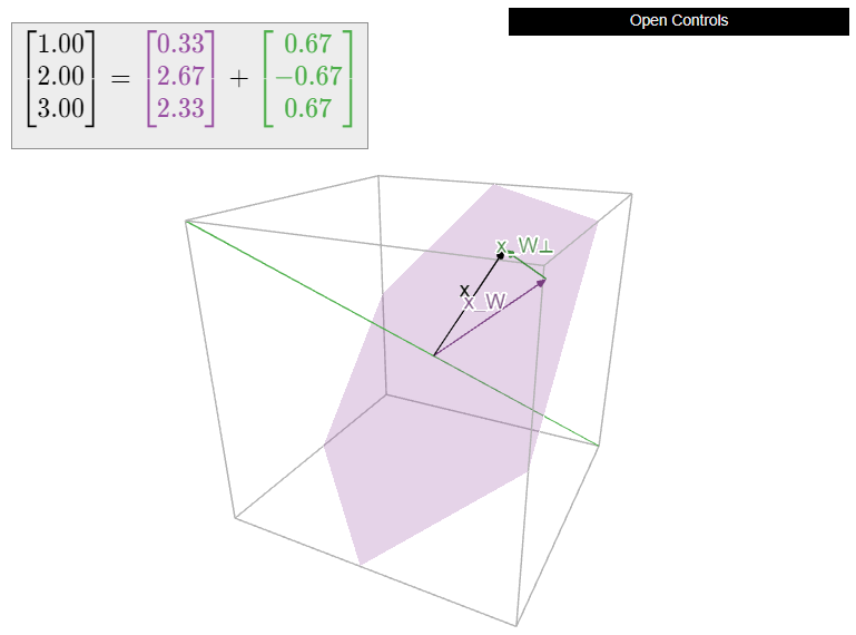
Let

$$W = \left\{\left(\begin{array}{c}x_1\\x_2\\x_3\end{array}\right)\bigm|x_1 - 2x_2 = x_3\right\} \quad\text{and}\quad x = \left(\begin{array}{c}1\\1\\1\end{array}\right). \nonumber$$

Compute $x_W$.

Solution

Method 1: First we need to find a spanning set for $W$. We notice that $W$ is the solution set of the homogeneous equation $x_1 - 2x_2 - x_3 = 0\text{,}$ so $W = \text{Nul}\left(\begin{array}{ccc}1&-2&-1\end{array}\right)$. We know how to compute a basis for a null space: we row reduce and find the parametric vector form. The matrix $\left(\begin{array}{ccc}1&-2&-1\end{array}\right)$ is already in reduced row echelon form. The parametric form is $x_1 = 2x_2 + x_3\text{,}$ so the parametric vector form is

$$\left(\begin{array}{c}x_1\\x_2\\x_3\end{array}\right) = x_2\left(\begin{array}{c}2\\1\\0\end{array}\right) + x_3\left(\begin{array}{c}1\\0\\1\end{array}\right), \nonumber$$

and hence a basis for $V$ is given by

$$\left\{\left(\begin{array}{c}2\\1\\0\end{array}\right),\;\left(\begin{array}{c}1\\0\\1\end{array}\right)\right\}. \nonumber$$

We let $A$ be the matrix whose columns are our basis vectors:

$$A = \left(\begin{array}{cc}2&1\\1&0\\0&1\end{array}\right). \nonumber$$

Hence $\text{Col}(A) = \text{Nul}\left(\begin{array}{ccc}1&-2&-1\end{array}\right) = W$.

Now we can continue with step 1 of the recipe. We compute

$$A^TA = \left(\begin{array}{cc}5&2\\2&2\end{array}\right) \qquad A^Tx = \left(\begin{array}{c}3\\2\end{array}\right). \nonumber$$

We write the linear system $A^TAc = A^Tx$ as an augmented matrix and row reduce:

$$\left(\begin{array}{cc|c}5&2&3\\2&2&2\end{array}\right)\xrightarrow{\text{RREF}}\left(\begin{array}{cc|c}1&0&1/3 \\ 0&1&2/3\end{array}\right). \nonumber$$

Hence we can take $c = {1/3\choose 2/3}\text{,}$ so

$$x_W = Ac =\left(\begin{array}{cc}2&1\\1&0\\0&1\end{array}\right)\left(\begin{array}{c}1/3\\2/3\end{array}\right) = \frac 13\left(\begin{array}{c}4\\1\\2\end{array}\right). \nonumber$$

Figure $\PageIndex{13}$: Orthogonal projection onto the plane $W$.

Method 2: In this case, it is easier to compute $x_{W^\perp}$. Indeed, since $W = \text{Nul}\left(\begin{array}{ccc}1&-2&-1\end{array}\right),$ the orthogonal complement is the line

$$V = W^\perp = \text{Col}\left(\begin{array}{c}1\\-2\\-1\end{array}\right). \nonumber$$

Using the formula for projection onto a line, Example $\PageIndex{7}$, gives

$$x_{W^\perp} = x_V = \frac{\left(\begin{array}{c}1\\1\\1\end{array}\right)\cdot\left(\begin{array}{c}1\\-2\\-1\end{array}\right)}{\left(\begin{array}{c}1\\-2\\-1\end{array}\right)\cdot\left(\begin{array}{c}1\\-2\\-1\end{array}\right)}\left(\begin{array}{c}1\\-2\\-1\end{array}\right)=\frac{1}{3}\left(\begin{array}{c}-1\\2\\1\end{array}\right). \nonumber$$

Hence we have

$$x_W = x - x_{W^\perp} = \left(\begin{array}{c}1\\1\\1\end{array}\right) - \frac 13\left(\begin{array}{c}-1\\2\\1\end{array}\right). = \frac 13\left(\begin{array}{c}4\\1\\2\end{array}\right), \nonumber$$

as above.

Example $\PageIndex{13}$: Projection onto a $3$-space in $\mathbb{R}^4$

Let

$$W = \text{Span}\left\{\left(\begin{array}{c}1\\0\\-1\\0\end{array}\right),\;\left(\begin{array}{c}0\\1\\0\\-1\end{array}\right),\;\left(\begin{array}{c}1\\1\\1\\-1\end{array}\right)\right\} \qquad x = \left(\begin{array}{c}0\\1\\3\\4\end{array}\right). \nonumber$$

Compute the orthogonal decomposition of $x$ with respect to $W$.

Solution

We have to solve the matrix equation $A^TAc = A^Tx\text{,}$ where

$$A = \left(\begin{array}{ccc}1&0&1\\0&1&1\\-1&0&1\\0&-1&-1\end{array}\right). \nonumber$$

We compute

$$A^TA = \left(\begin{array}{ccc}2&0&0\\0&2&2\\0&2&4\end{array}\right) \qquad A^Tx = \left(\begin{array}{c}-3\\3\\0\end{array}\right). \nonumber$$

We form an augmented matrix and row reduce:

$$\left(\begin{array}{ccc|c}2&0&0&-3\\0&2&2&-3\\0&2&4&0\end{array}\right)\xrightarrow{\text{RREF}}\left(\begin{array}{ccc|c}1&0&0&-3/2 \\ 0&1&0&-3\\0&0&1&3/2\end{array}\right) \implies c = \frac 12\left(\begin{array}{c}-3\\-6\\3\end{array}\right). \nonumber$$

It follows that

$$x_W = Ac = \frac 12\left(\begin{array}{c}0\\-3\\6\\3\end{array}\right) \qquad x_{W^\perp} = \frac 12\left(\begin{array}{c}0\\5\\0\\5\end{array}\right). \nonumber$$

In the context of the above recipe, if we start with a basis of $W\text{,}$ then it turns out that the square matrix $A^TA$ is automatically invertible! (It is always the case that $A^TA$ is square and the equation $A^TAc = A^Tx$ is consistent, but $A^TA$ need not be invertible in general.)

Corollary $\PageIndex{1}$

Let $A$ be an $m \times n$ matrix with linearly independent columns and let $W = \text{Col}(A)$. Then the $n\times n$ matrix $A^TA$ is invertible, and for all vectors $x$ in $\mathbb{R}^m \text{,}$ we have

$$x_W = A(A^TA)^{-1} A^Tx. \nonumber$$

Proof

We will show that $\text{Nul}(A^TA)=\{0\}\text{,}$ which implies invertibility by Theorem 5.1.1 in Section 5.1. Suppose that $A^TAc = 0$. Then $A^TAc = A^T0\text{,}$ so $0_W = Ac$ by Theorem $\PageIndex{2}$. But $0_W = 0$ (the orthogonal decomposition of the zero vector is just $0 = 0 + 0)\text{,}$ so $Ac = 0\text{,}$ and therefore $c$ is in $\text{Nul}(A)$. Since the columns of $A$ are linearly independent, we have $c=0\text{,}$ so $\text{Nul}(A^TA)=0\text{,}$ as desired.

Let $x$ be a vector in $\mathbb{R}^n$ and let $c$ be a solution of $A^TAc = A^Tx$. Then $c = (A^TA)^{-1} A^Tx\text{,}$ so $x_W =Ac = A(A^TA)^{-1} A^Tx$.

The corollary applies in particular to the case where we have a subspace $W$ of $\mathbb{R}^m \text{,}$ and a basis $v_1,v_2,\ldots,v_n$ for $W$. To apply the corollary, we take $A$ to be the $m\times n$ matrix with columns $v_1,v_2,\ldots,v_n$.

Example $\PageIndex{14}$: Computing a projection

Continuing with the above Example $\PageIndex{11}$, let

$$W = \text{Span}\left\{\left(\begin{array}{c}1\\0\\-1\end{array}\right),\;\left(\begin{array}{c}1\\1\\0\end{array}\right)\right\} \qquad x = \left(\begin{array}{c}x_1\\x_2\\x_3\end{array}\right). \nonumber$$

Compute $x_W$ using the formula $x_W = A(A^TA)^{-1} A^Tx$.

Solution

Clearly the spanning vectors are noncollinear, so according to Corollary $\PageIndex{1}$, we have $x_W = A(A^TA)^{-1} A^Tx\text{,}$ where

$$A = \left(\begin{array}{cc}1&1\\0&1\\-1&0\end{array}\right). \nonumber$$

We compute

$$A^TA = \left(\begin{array}{cc}2&1\\1&2\end{array}\right) \implies (A^TA)^{-1} = \frac 13\left(\begin{array}{cc}2&-1\\-1&2\end{array}\right), \nonumber$$

so

$$\begin{aligned}x_{W}&=A(A^TA)^{-1}A^Tx=\left(\begin{array}{cc}1&1\\0&1\\-1&0\end{array}\right)\frac{1}{3}\left(\begin{array}{cc}2&-1\\-1&2\end{array}\right)\left(\begin{array}{ccc}1&0&-1\\1&1&0\end{array}\right)\left(\begin{array}{c}x_1\\x_2\\x_3\end{array}\right) \\ &=\frac{1}{3}\left(\begin{array}{ccc}2&1&-1\\1&2&1\\-1&1&2\end{array}\right)\left(\begin{array}{c}x_1\\x_2\\x_3\end{array}\right)=\frac{1}{3}\left(\begin{array}{rrrrr} 2x_1 &+& x_2 &-& x_3\\ x_1 &+& 2x_2 &+& x_3\\ -x_1 &+& x_2 &+& 2x_3\end{array}\right).\end{aligned}$$

So, for example, if $x=(1,0,0)\text{,}$ this formula tells us that $x_W = (2,1,-1)$.

Orthogonal Projection

In this subsection, we change perspective and think of the orthogonal projection $x_W$ as a function of $x$. This function turns out to be a linear transformation with many nice properties, and is a good example of a linear transformation which is not originally defined as a matrix transformation.

Proposition $\PageIndex{1}$: Properties of Orthogonal Projections

Let $W$ be a subspace of $\mathbb{R}^n \text{,}$ and define $T\colon\mathbb{R}^n \to\mathbb{R}^n$ by $T(x) = x_W$. Then:

1. $T$ is a linear transformation.
2. $T(x)=x$ if and only if $x$ is in $W$.
3. $T(x)=0$ if and only if $x$ is in $W^\perp$.
4. $T\circ T = T$.
5. The range of $T$ is $W$.

Proof

1. We have to verify the defining properties of linearity, Definition 3.3.1 in Section 3.3. Let $x,y$ be vectors in $\mathbb{R}^n \text{,}$ and let $x = x_W + x_{W^\perp}$ and $y = y_W + y_{W^\perp}$ be their orthogonal decompositions. Since $W$ and $W^\perp$ are subspaces, the sums $x_W+y_W$ and $x_{W^\perp}+y_{W^\perp}$ are in $W$ and $W^\perp\text{,}$ respectively. Therefore, the orthogonal decomposition of $x+y$ is $(x_W+y_W)+(x_{W^\perp}+y_{W^\perp})\text{,}$ so $$T(x+y) = (x+y)_W = x_W+y_W = T(x) + T(y). \nonumber$$ Now let $c$ be a scalar. Then $cx_W$ is in $W$ and $cx_{W^\perp}$ is in $W^\perp\text{,}$ so the orthogonal decomposition of $cx$ is $cx_W + cx_{W^\perp}\text{,}$ and therefore, $$T(cx) = (cx)_W = cx_W = cT(x). \nonumber$$ Since $T$ satisfies the two defining properties, Definition 3.3.1 in Section 3.3, it is a linear transformation.
2. See Example $\PageIndex{2}$.
3. See Example $\PageIndex{3}$.
4. For any $x$ in $\mathbb{R}^n$ the vector $T(x)$ is in $W\text{,}$ so $T\circ T(x) = T(T(x)) = T(x)$ by 2. Any vector $x$ in $W$ is in the range of $T\text{,}$ because $T(x) = x$ for such vectors. On the other hand, for any vector $x$ in $\mathbb{R}^n$ the output $T(x) = x_W$ is in $W\text{,}$ so $W$ is the range of $T$.

We compute the standard matrix of the orthogonal projection in the same way as for any other transformation, Theorem 3.3.1 in Section 3.3: by evaluating on the standard coordinate vectors. In this case, this means projecting the standard coordinate vectors onto the subspace.

Example $\PageIndex{15}$: Matrix of a projection

Let $L$ be the line in $\mathbb{R}^2$ spanned by the vector $u = {3\choose 2}\text{,}$ and define $T\colon\mathbb{R}^2 \to\mathbb{R}^2$ by $T(x)=x_L$. Compute the standard matrix $B$ for $T$.

Solution

The columns of $B$ are $T(e_1) = (e_1)_L$ and $T(e_2) = (e_2)_L$. We have

$$\left.\begin{aligned}(e_1)_{L}&=\frac{u\cdot e_1}{u\cdot u} \quad u=\frac{3}{13}\left(\begin{array}{c}3\\2\end{array}\right) \\ (e_2)_{L}&=\frac{u\cdot e_2}{u\cdot u}\quad u=\frac{2}{13}\left(\begin{array}{c}3\\2\end{array}\right)\end{aligned}\right\}\quad\implies\quad B=\frac{1}{13}\left(\begin{array}{cc}9&6\\6&4\end{array}\right).\nonumber$$

Example $\PageIndex{16}$: Matrix of a projection

Let $L$ be the line in $\mathbb{R}^2$ spanned by the vector

$$u = \left(\begin{array}{c}-1\\1\\1\end{array}\right), \nonumber$$

and define $T\colon\mathbb{R}^3 \to\mathbb{R}^3$ by $T(x)=x_L$. Compute the standard matrix $B$ for $T$.

Solution

The columns of $B$ are $T(e_1) = (e_1)_L\text{,}$ $T(e_2) = (e_2)_L\text{,}$ and $T(e_3) = (e_3)_L$. We have

$$\left. \begin{split} (e_1)_L \amp= \frac{u\cdot e_1}{u\cdot u}\quad u = \frac{-1}{3}\left(\begin{array}{c}-1\\1\\1\end{array}\right) \\ (e_2)_L \amp= \frac{u\cdot e_2}{u\cdot u}\quad u = \frac{1}{3}\left(\begin{array}{c}-1\\1\\1\end{array}\right) \\ (e_3)_L \amp= \frac{u\cdot e_3}{u\cdot u}\quad u = \frac{1}{3}\left(\begin{array}{c}-1\\1\\1\end{array}\right) \end{split} \right\} \quad\implies\quad B = \frac 1{3}\left(\begin{array}{ccc}1&-1&-1\\-1&1&1\\-1&1&1\end{array}\right). \nonumber$$

Example $\PageIndex{17}$: Matrix of a projection

Continuing with Example $\PageIndex{11}$, let

$$W = \text{Span}\left\{\left(\begin{array}{c}1\\0\\-1\end{array}\right),\;\left(\begin{array}{c}1\\1\\0\end{array}\right)\right\}, \nonumber$$

and define $T\colon\mathbb{R}^3 \to\mathbb{R}^3$ by $T(x)=x_W$. Compute the standard matrix $B$ for $T$.

Solution

The columns of $B$ are $T(e_1) = (e_1)_W\text{,}$ $T(e_2) = (e_2)_W\text{,}$ and $T(e_3) = (e_3)_W$. Let

$$A = \left(\begin{array}{cc}1&1\\0&1\\-1&0\end{array}\right). \nonumber$$

To compute each $(e_i)_W\text{,}$ we solve the matrix equation $A^TAc = A^Te_i$ for $c\text{,}$ then use the equality $(e_i)_W = Ac$. First we note that

$$A^TA = \left(\begin{array}{cc}2&1\\1&2\end{array}\right); \qquad A^Te_i = \text{the $i$th column of } A^T = \left(\begin{array}{ccc}1&0&-1\\1&1&0\end{array}\right). \nonumber$$

For $e_1\text{,}$ we form an augmented matrix and row reduce:

$$\left(\begin{array}{cc|c}2&1&1\\1&2&1\end{array}\right)\xrightarrow{\text{RREF}} \left(\begin{array}{cc|c}1&0&1/3 \\ 0&1&1/3\end{array}\right) \implies (e_1)_W = A\left(\begin{array}{c}1/3 \\ 1/3\end{array}\right) = \frac 13\left(\begin{array}{c}2\\1\\-1\end{array}\right). \nonumber$$

We do the same for $e_2\text{:}$

$$\left(\begin{array}{cc|c}2&1&0\\1&2&1\end{array}\right)\xrightarrow{\text{RREF}}\left(\begin{array}{cc|c}1&0&-1/3 \\ 0&1&2/3\end{array}\right) \implies (e_1)_W = A\left(\begin{array}{c}-1/3 \\ 2/3\end{array}\right) = \frac 13\left(\begin{array}{c}1\\2\\1\end{array}\right) \nonumber$$

and for $e_3\text{:}$

$$\left(\begin{array}{cc|c}2&1&-1\\1&2&0\end{array}\right)\xrightarrow{\text{RREF}}\left(\begin{array}{cc|c}1&0&-2/3 \\ 0&1&1/3\end{array}\right) \implies (e_1)_W = A\left(\begin{array}{c}-2/3 \\ 1/3\end{array}\right) = \frac 13\left(\begin{array}{c}-1\\1\\2\end{array}\right). \nonumber$$

It follows that

$$B = \frac 13\left(\begin{array}{ccc}2&1&-1\\1&2&1\\-1&1&2\end{array}\right). \nonumber$$

In the previous Example $\PageIndex{17}$, we could have used the fact that

$$\left\{\left(\begin{array}{c}1\\0\\-1\end{array}\right),\;\left(\begin{array}{c}1\\1\\0\end{array}\right)\right\} \nonumber$$

forms a basis for $W\text{,}$ so that

$$T(x) = x_W = \bigl[A(A^TA)^{-1} A^T\bigr]x \quad\text{for}\quad A = \left(\begin{array}{cc}1&1\\0&1\\-1&0\end{array}\right) \nonumber$$

by the Corollary $\PageIndex{1}$. In this case, we have already expressed $T$ as a matrix transformation with matrix $A(A^TA)^{-1} A^T$. See this Example $\PageIndex{14}$.

Note $\PageIndex{2}$

Let $W$ be a subspace of $\mathbb{R}^n$ with basis $v_1,v_2,\ldots,v_m\text{,}$ and let $A$ be the matrix with columns $v_1,v_2,\ldots,v_m$. Then the standard matrix for $T(x) = x_W$ is

$$A(A^TA)^{-1} A^T. \nonumber$$

We can translate the above properties of orthogonal projections, Proposition $\PageIndex{1}$, into properties of the associated standard matrix.

Proposition $\PageIndex{2}$: Properties of Projection Matrices

Let $W$ be a subspace of $\mathbb{R}^n \text{,}$ define $T\colon\mathbb{R}^n \to\mathbb{R}^n$ by $T(x) = x_W\text{,}$ and let $B$ be the standard matrix for $T$. Then:

1. $\text{Col}(B) = W.$
2. $\text{Nul}(B) = W^\perp.$
3. $B^2 = B.$
4. If $W \neq \{0\}\text{,}$ then 1 is an eigenvalue of $B$ and the 1-eigenspace for $B$ is $W$.
5. If $W \neq \mathbb{R}^n \text{,}$ then 0 is an eigenvalue of $B$ and the 0-eigenspace for $B$ is $W^\perp$.
6. $B$ is similar to the diagonal matrix with $m$ ones and $n-m$ zeros on the diagonal, where $m = \dim(W).$

Proof

The first four assertions are translations of properties 5, 3, 4, and 2 from Proposition $\PageIndex{2}$, respectively, using this Note 3.1.1 in Section 3.1 and Theorem 3.4.1 in Section 3.4. The fifth assertion is equivalent to the second, by Fact 5.1.2 in Section 5.1.

For the final assertion, we showed in the proof of this Theorem $\PageIndex{1}$ that there is a basis of $\mathbb{R}^n$ of the form $\{v_1,\ldots,v_m,v_{m+1},\ldots,v_n\}\text{,}$ where $\{v_1,\ldots,v_m\}$ is a basis for $W$ and $\{v_{m+1},\ldots,v_n\}$ is a basis for $W^\perp$. Each $v_i$ is an eigenvector of $B\text{:}$ indeed, for $i\leq m$ we have

$$Bv_i = T(v_i) = v_i = 1\cdot v_i \nonumber$$

because $v_i$ is in $W\text{,}$ and for $i > m$ we have

$$Bv_i = T(v_i) = 0 = 0\cdot v_i \nonumber$$

because $v_i$ is in $W^\perp$. Therefore, we have found a basis of eigenvectors, with associated eigenvalues $1,\ldots,1,0,\ldots,0$ ($m$ ones and $n-m$ zeros). Now we use Theorem 5.4.1 in Section 5.4.

We emphasize that the properties of projection matrices, Proposition $\PageIndex{2}$, would be very hard to prove in terms of matrices. By translating all of the statements into statements about linear transformations, they become much more transparent. For example, consider the projection matrix we found in Example $\PageIndex{17}$. Just by looking at the matrix it is not at all obvious that when you square the matrix you get the same matrix back.

Example $\PageIndex{18}$

Continuing with above Example $\PageIndex{17}$, we showed that

$$B = \frac 13\left(\begin{array}{ccc}2&1&-1\\1&2&1\\-1&1&2\end{array}\right) \nonumber$$

is the standard matrix of the orthogonal projection onto

$$W = \text{Span}\left\{\left(\begin{array}{c}1\\0\\-1\end{array}\right),\;\left(\begin{array}{c}1\\1\\0\end{array}\right)\right\}. \nonumber$$

One can verify by hand that $B^2=B$ (try it!). We compute $W^\perp$ as the null space of

$$\left(\begin{array}{ccc}1&0&-1\\1&1&0\end{array}\right)\xrightarrow{\text{RREF}}\left(\begin{array}{ccc}1&0&-1\\0&1&1\end{array}\right). \nonumber$$

The free variable is $x_3\text{,}$ and the parametric form is $x_1 = x_3,\,x_2 = -x_3\text{,}$ so that

$$W^\perp = \text{Span}\left\{\left(\begin{array}{c}1\\-1\\1\end{array}\right)\right\}. \nonumber$$

It follows that $B$ has eigenvectors

$$\left(\begin{array}{c}1\\0\\-1\end{array}\right),\qquad \left(\begin{array}{c}1\\1\\0\end{array}\right),\qquad \left(\begin{array}{c}1\\-1\\1\end{array}\right) \nonumber$$

with eigenvalues $1,1,0\text{,}$ respectively, so that

$$B = \left(\begin{array}{ccc}1&1&1\\0&1&-1\\-1&0&1\end{array}\right)\left(\begin{array}{ccc}1&0&0\\0&1&0\\0&0&0\end{array}\right)\left(\begin{array}{ccc}1&1&1\\0&1&-1\\-1&0&1\end{array}\right)^{-1}. \nonumber$$

Remark

As we saw in Example $\PageIndex{18}$, if you are willing to compute bases for $W$ and $W^\perp\text{,}$ then this provides a third way of finding the standard matrix $B$ for projection onto $W\text{:}$ indeed, if $\{v_1,v_2,\ldots,v_m\}$ is a basis for $W$ and $\{v_{m+1},v_{m+2},\ldots,v_n\}$ is a basis for $W^\perp\text{,}$ then

$$B=\left(\begin{array}{cccc}|&|&\quad&| \\ v_1&v_2&\cdots&v_n\\ |&|&\quad&| \end{array}\right)\left(\begin{array}{cccccc}1&\cdots &0&0&\cdots &0 \\ \vdots&\ddots&\vdots&\vdots&\ddots&\vdots \\ 0&\cdots&1&0&\cdots&0\\0&\cdots&0&0&\cdots&0\\ \vdots&\ddots&\vdots&\vdots&\ddots&\vdots \\ 0&\cdots&0&0&\cdots&0\end{array}\right)\left(\begin{array}{cccc}|&|&\quad&| \\ v_1&v_1&\cdots&v_n \\ |&|&\quad&|\end{array}\right)^{-1},\nonumber$$

where the middle matrix in the product is the diagonal matrix with $m$ ones and $n-m$ zeros on the diagonal. However, since you already have a basis for $W\text{,}$ it is faster to multiply out the expression $A(A^TA)^{-1} A^T$ as in Corollary $\PageIndex{1}$.

Remark: Reflections

Let $W$ be a subspace of $\mathbb{R}^n \text{,}$ and let $x$ be a vector in $\mathbb{R}^n$. The reflection of $x$ over $W$ is defined to be the vector

$$\text{ref}_W(x) = x - 2x_{W^\perp}. \nonumber$$

In other words, to find $\text{ref}_W(x)$ one starts at $x\text{,}$ then moves to $x-x_{W^\perp} = x_W\text{,}$ then continues in the same direction one more time, to end on the opposite side of $W$.

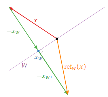
Figure $\PageIndex{14}$

Since $x_{W^\perp} = x - x_W\text{,}$ we also have

$$\text{ref}_W(x) = x - 2(x - x_W) = 2x_W - x. \nonumber$$

We leave it to the reader to check using the definition that:

1. $\text{ref}_W\circ\text{ref}_W = \text{Id}_{\mathbb{R}^n }.$
2. The $1$-eigenspace of $\text{ref}_W$ is $W\text{,}$ and the $-1$-eigenspace of $\text{ref}_W$ is $W^\perp$.
3. $\text{ref}_W$ is similar to the diagonal matrix with $m = \dim(W)$ ones on the diagonal and $n-m$ negative ones.