6: Orthogonality

Last updated
Save as PDF

Page ID: 70211

$ \newcommand{\vecs}[1]{\overset { \scriptstyle \rightharpoonup} {\mathbf{#1}} } $ $ \newcommand{\vecd}[1]{\overset{-\!-\!\rightharpoonup}{\vphantom{a}\smash {#1}}} $$\newcommand{\id}{\mathrm{id}}$ $ \newcommand{\Span}{\mathrm{span}}$ $ \newcommand{\kernel}{\mathrm{null}\,}$ $ \newcommand{\range}{\mathrm{range}\,}$ $ \newcommand{\RealPart}{\mathrm{Re}}$ $ \newcommand{\ImaginaryPart}{\mathrm{Im}}$ $ \newcommand{\Argument}{\mathrm{Arg}}$ $ \newcommand{\norm}[1]{\| #1 \|}$ $ \newcommand{\inner}[2]{\langle #1, #2 \rangle}$ $ \newcommand{\Span}{\mathrm{span}}$ $\newcommand{\id}{\mathrm{id}}$ $ \newcommand{\Span}{\mathrm{span}}$ $ \newcommand{\kernel}{\mathrm{null}\,}$ $ \newcommand{\range}{\mathrm{range}\,}$ $ \newcommand{\RealPart}{\mathrm{Re}}$ $ \newcommand{\ImaginaryPart}{\mathrm{Im}}$ $ \newcommand{\Argument}{\mathrm{Arg}}$ $ \newcommand{\norm}[1]{\| #1 \|}$ $ \newcommand{\inner}[2]{\langle #1, #2 \rangle}$ $ \newcommand{\Span}{\mathrm{span}}$$\newcommand{\AA}{\unicode[.8,0]{x212B}}$

Let us recall one last time the structure of this book:

Solve the matrix equation $Ax=b$.
Solve the matrix equation $Ax=\lambda x\text{,}$ where $\lambda$ is a number.
Approximately solve the matrix equation $Ax=b$.

We have now come to the third part.

Note $\PageIndex{1}$

Approximately solve the matrix equation $Ax=b.$

Finding approximate solutions of equations generally requires computing the closest vector on a subspace to a given vector. This becomes an orthogonality problem: one needs to know which vectors are perpendicular to the subspace.

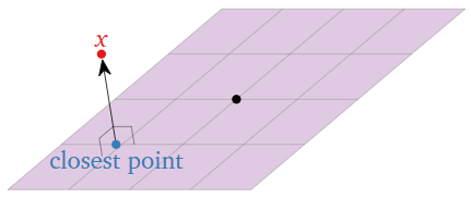
$clipboard_e4c312e06d8c1c7b40ae1ce8dfa3f77e5.png$

Figure $\PageIndex{1}$

First we will define orthogonality and learn to find orthogonal complements of subspaces in Section 6.1 and Section 6.2. The core of this chapter is Section 6.3, in which we discuss the orthogonal projection of a vector onto a subspace; this is a method of calculating the closest vector on a subspace to a given vector. These calculations become easier in the presence of an orthogonal set, as we will see in Section 6.4. In Section 6.5 we will present the least-squares method of approximately solving systems of equations, and we will give applications to data modeling.

Example $\PageIndex{1}$

In data modeling, one often asks: “what line is my data supposed to lie on?” This can be solved using a simple application of the least-squares method.

$clipboard_e9c04a2611d7045928bccedd7ad9c0a17.png$

Figure $\PageIndex{2}$

Example $\PageIndex{2}$

Gauss invented the method of least squares to find a best-fit ellipse: he correctly predicted the (elliptical) orbit of the asteroid Ceres as it passed behind the sun in 1801.

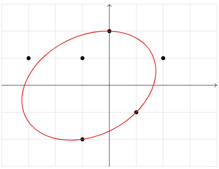
$clipboard_e8ec747dcd6cf56fd41cfcac28daede0f.png$

Figure $\PageIndex{3}$

6.1: Dot Products and Orthogonality
In this chapter, it will be necessary to find the closest point on a subspace to a given point. The closest point has the property that the difference between the two points is orthogonal, or perpendicular, to the subspace. For this reason, we need to develop notions of orthogonality, length, and distance.
6.2: Orthogonal Complements
It will be important to compute the set of all vectors that are orthogonal to a given set of vectors. It turns out that a vector is orthogonal to a set of vectors if and only if it is orthogonal to the span of those vectors, which is a subspace, so we restrict ourselves to the case of subspaces.
6.3: Orthogonal Projection
Let W be a subspace of Rn and let x be a vector in Rn . In this section, we will learn to compute the closest vector xW to x in W. The vector xW is called the orthogonal projection of x onto W . This is exactly what we will use to almost solve matrix equations.
6.4: Orthogonal Sets
6.5: The Method of Least Squares

Search

Note \(\PageIndex{1}\)

Example \(\PageIndex{1}\)

Example \(\PageIndex{2}\)