
6.5: The Method of Least Squares
- Page ID
- 79396

\( \newcommand{\vecs}[1]{\overset { \scriptstyle \rightharpoonup} {\mathbf{#1}} } \)
\( \newcommand{\vecd}[1]{\overset{-\!-\!\rightharpoonup}{\vphantom{a}\smash {#1}}} \)
\( \newcommand{\dsum}{\displaystyle\sum\limits} \)
\( \newcommand{\dint}{\displaystyle\int\limits} \)
\( \newcommand{\dlim}{\displaystyle\lim\limits} \)
\( \newcommand{\id}{\mathrm{id}}\) \( \newcommand{\Span}{\mathrm{span}}\)
( \newcommand{\kernel}{\mathrm{null}\,}\) \( \newcommand{\range}{\mathrm{range}\,}\)
\( \newcommand{\RealPart}{\mathrm{Re}}\) \( \newcommand{\ImaginaryPart}{\mathrm{Im}}\)
\( \newcommand{\Argument}{\mathrm{Arg}}\) \( \newcommand{\norm}[1]{\| #1 \|}\)
\( \newcommand{\inner}[2]{\langle #1, #2 \rangle}\)
\( \newcommand{\Span}{\mathrm{span}}\)
\( \newcommand{\id}{\mathrm{id}}\)
\( \newcommand{\Span}{\mathrm{span}}\)
\( \newcommand{\kernel}{\mathrm{null}\,}\)
\( \newcommand{\range}{\mathrm{range}\,}\)
\( \newcommand{\RealPart}{\mathrm{Re}}\)
\( \newcommand{\ImaginaryPart}{\mathrm{Im}}\)
\( \newcommand{\Argument}{\mathrm{Arg}}\)
\( \newcommand{\norm}[1]{\| #1 \|}\)
\( \newcommand{\inner}[2]{\langle #1, #2 \rangle}\)
\( \newcommand{\Span}{\mathrm{span}}\) \( \newcommand{\AA}{\unicode[.8,0]{x212B}}\)
\( \newcommand{\vectorA}[1]{\vec{#1}} % arrow\)
\( \newcommand{\vectorAt}[1]{\vec{\text{#1}}} % arrow\)
\( \newcommand{\vectorB}[1]{\overset { \scriptstyle \rightharpoonup} {\mathbf{#1}} } \)
\( \newcommand{\vectorC}[1]{\textbf{#1}} \)
\( \newcommand{\vectorD}[1]{\overrightarrow{#1}} \)
\( \newcommand{\vectorDt}[1]{\overrightarrow{\text{#1}}} \)
\( \newcommand{\vectE}[1]{\overset{-\!-\!\rightharpoonup}{\vphantom{a}\smash{\mathbf {#1}}}} \)
\( \newcommand{\vecs}[1]{\overset { \scriptstyle \rightharpoonup} {\mathbf{#1}} } \)
\(\newcommand{\longvect}{\overrightarrow}\)
\( \newcommand{\vecd}[1]{\overset{-\!-\!\rightharpoonup}{\vphantom{a}\smash {#1}}} \)
\(\newcommand{\avec}{\mathbf a}\) \(\newcommand{\bvec}{\mathbf b}\) \(\newcommand{\cvec}{\mathbf c}\) \(\newcommand{\dvec}{\mathbf d}\) \(\newcommand{\dtil}{\widetilde{\mathbf d}}\) \(\newcommand{\evec}{\mathbf e}\) \(\newcommand{\fvec}{\mathbf f}\) \(\newcommand{\nvec}{\mathbf n}\) \(\newcommand{\pvec}{\mathbf p}\) \(\newcommand{\qvec}{\mathbf q}\) \(\newcommand{\svec}{\mathbf s}\) \(\newcommand{\tvec}{\mathbf t}\) \(\newcommand{\uvec}{\mathbf u}\) \(\newcommand{\vvec}{\mathbf v}\) \(\newcommand{\wvec}{\mathbf w}\) \(\newcommand{\xvec}{\mathbf x}\) \(\newcommand{\yvec}{\mathbf y}\) \(\newcommand{\zvec}{\mathbf z}\) \(\newcommand{\rvec}{\mathbf r}\) \(\newcommand{\mvec}{\mathbf m}\) \(\newcommand{\zerovec}{\mathbf 0}\) \(\newcommand{\onevec}{\mathbf 1}\) \(\newcommand{\real}{\mathbb R}\) \(\newcommand{\twovec}[2]{\left[\begin{array}{r}#1 \\ #2 \end{array}\right]}\) \(\newcommand{\ctwovec}[2]{\left[\begin{array}{c}#1 \\ #2 \end{array}\right]}\) \(\newcommand{\threevec}[3]{\left[\begin{array}{r}#1 \\ #2 \\ #3 \end{array}\right]}\) \(\newcommand{\cthreevec}[3]{\left[\begin{array}{c}#1 \\ #2 \\ #3 \end{array}\right]}\) \(\newcommand{\fourvec}[4]{\left[\begin{array}{r}#1 \\ #2 \\ #3 \\ #4 \end{array}\right]}\) \(\newcommand{\cfourvec}[4]{\left[\begin{array}{c}#1 \\ #2 \\ #3 \\ #4 \end{array}\right]}\) \(\newcommand{\fivevec}[5]{\left[\begin{array}{r}#1 \\ #2 \\ #3 \\ #4 \\ #5 \\ \end{array}\right]}\) \(\newcommand{\cfivevec}[5]{\left[\begin{array}{c}#1 \\ #2 \\ #3 \\ #4 \\ #5 \\ \end{array}\right]}\) \(\newcommand{\mattwo}[4]{\left[\begin{array}{rr}#1 \amp #2 \\ #3 \amp #4 \\ \end{array}\right]}\) \(\newcommand{\laspan}[1]{\text{Span}\{#1\}}\) \(\newcommand{\bcal}{\cal B}\) \(\newcommand{\ccal}{\cal C}\) \(\newcommand{\scal}{\cal S}\) \(\newcommand{\wcal}{\cal W}\) \(\newcommand{\ecal}{\cal E}\) \(\newcommand{\coords}[2]{\left\{#1\right\}_{#2}}\) \(\newcommand{\gray}[1]{\color{gray}{#1}}\) \(\newcommand{\lgray}[1]{\color{lightgray}{#1}}\) \(\newcommand{\rank}{\operatorname{rank}}\) \(\newcommand{\row}{\text{Row}}\) \(\newcommand{\col}{\text{Col}}\) \(\renewcommand{\row}{\text{Row}}\) \(\newcommand{\nul}{\text{Nul}}\) \(\newcommand{\var}{\text{Var}}\) \(\newcommand{\corr}{\text{corr}}\) \(\newcommand{\len}[1]{\left|#1\right|}\) \(\newcommand{\bbar}{\overline{\bvec}}\) \(\newcommand{\bhat}{\widehat{\bvec}}\) \(\newcommand{\bperp}{\bvec^\perp}\) \(\newcommand{\xhat}{\widehat{\xvec}}\) \(\newcommand{\vhat}{\widehat{\vvec}}\) \(\newcommand{\uhat}{\widehat{\uvec}}\) \(\newcommand{\what}{\widehat{\wvec}}\) \(\newcommand{\Sighat}{\widehat{\Sigma}}\) \(\newcommand{\lt}{<}\) \(\newcommand{\gt}{>}\) \(\newcommand{\amp}{&}\) \(\definecolor{fillinmathshade}{gray}{0.9}\)- Learn examples of best-fit problems.
- Learn to turn a best-fit problem into a least-squares problem.
- Recipe: find a least-squares solution (two ways). solution.
- Picture: geometry of a least-squares solution.
- Vocabulary words: least-squares solution.
In this section, we answer the following important question:
Suppose that \(Ax=b\) does not have a solution. What is the best approximate solution?
For our purposes, the best approximate solution is called the least-squares solution. We will present two methods for finding least-squares solutions, and we will give several applications to best-fit problems.
Least-Squares Solutions
We begin by clarifying exactly what we will mean by a “best approximate solution” to an inconsistent matrix equation \(Ax=b\).
Let \(A\) be an \(m\times n\) matrix and let \(b\) be a vector in \(\mathbb{R}^m \). A least-squares solution of the matrix equation \(Ax=b\) is a vector \(\hat x\) in \(\mathbb{R}^n \) such that
\[ \text{dist}(b,\,A\hat x) \leq \text{dist}(b,\,Ax) \nonumber \]
for all other vectors \(x\) in \(\mathbb{R}^n \).
Recall that \(\text{dist}(v,w) = \|v-w\|\) is the distance, Definition 6.1.2 in Section 6.1, between the vectors \(v\) and \(w\). The term “least squares” comes from the fact that \(\text{dist}(b,Ax) = \|b-A\hat x\|\) is the square root of the sum of the squares of the entries of the vector \(b-A\hat x\). So a least-squares solution minimizes the sum of the squares of the differences between the entries of \(A\hat x\) and \(b\). In other words, a least-squares solution solves the equation \(Ax=b\) as closely as possible, in the sense that the sum of the squares of the difference \(b-Ax\) is minimized.
Least Squares: Picture
Suppose that the equation \(Ax=b\) is inconsistent. Recall from Note 2.3.6 in Section 2.3 that the column space of \(A\) is the set of all other vectors \(c\) such that \(Ax=c\) is consistent. In other words, \(\text{Col}(A)\) is the set of all vectors of the form \(Ax.\) Hence, the closest vector, Note 6.3.1 in Section 6.3, of the form \(Ax\) to \(b\) is the orthogonal projection of \(b\) onto \(\text{Col}(A)\). This is denoted \(b_{\text{Col}(A)}\text{,}\) following Definition 6.3.1 in Section 6.3.
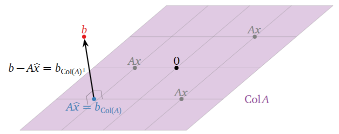
Figure \(\PageIndex{1}\)
A least-squares solution of \(Ax=b\) is a solution \(\hat x\) of the consistent equation \(Ax=b_{\text{Col}(A)}\)
If \(Ax=b\) is consistent, then \(b_{\text{Col}(A)} = b\text{,}\) so that a least-squares solution is the same as a usual solution.
Where is \(\hat x\) in this picture? If \(v_1,v_2,\ldots,v_n\) are the columns of \(A\text{,}\) then
\[ A\hat x = A\left(\begin{array}{c}\hat{x}_1 \\ \hat{x}_2 \\ \vdots \\ \hat{x}_{n}\end{array}\right) = \hat x_1v_1 + \hat x_2v_2 + \cdots + \hat x_nv_n. \nonumber \]
Hence the entries of \(\hat x\) are the “coordinates” of \(b_{\text{Col}(A)}\) with respect to the spanning set \(\{v_1,v_2,\ldots,v_m\}\) of \(\text{Col}(A)\). (They are honest \(\mathcal{B}\)-coordinates if the columns of \(A\) are linearly independent.)
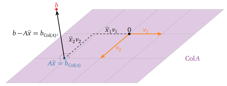
Figure \(\PageIndex{2}\)
We learned to solve this kind of orthogonal projection problem in Section 6.3.
Let \(A\) be an \(m\times n\) matrix and let \(b\) be a vector in \(\mathbb{R}^m \). The least-squares solutions of \(Ax=b\) are the solutions of the matrix equation
\[ A^TAx = A^Tb \nonumber \]
- Proof
-
By Theorem 6.3.2 in Section 6.3, if \(\hat x\) is a solution of the matrix equation \(A^TAx = A^Tb\text{,}\) then \(A\hat x\) is equal to \(b_{\text{Col}(A)}\). We argued above that a least-squares solution of \(Ax=b\) is a solution of \(Ax = b_{\text{Col}(A)}.\)
In particular, finding a least-squares solution means solving a consistent system of linear equations. We can translate the above theorem into a recipe:
Let \(A\) be an \(m\times n\) matrix and let \(b\) be a vector in \(\mathbb{R}^n \). Here is a method for computing a least-squares solution of \(Ax=b\text{:}\)
- Compute the matrix \(A^TA\) and the vector \(A^Tb\).
- Form the augmented matrix for the matrix equation \(A^TAx = A^Tb\text{,}\) and row reduce.
- This equation is always consistent, and any solution \(\hat x\) is a least-squares solution.
To reiterate: once you have found a least-squares solution \(\hat x\) of \(Ax=b\text{,}\) then \(b_{\text{Col}(A)}\) is equal to \(A\hat x\).
Find the least-squares solutions of \(Ax=b\) where:
\[ A = \left(\begin{array}{cc}0&1\\1&1\\2&1\end{array}\right) \qquad b = \left(\begin{array}{c}6\\0\\0\end{array}\right). \nonumber \]
What quantity is being minimized?
Solution
We have
\[ A^TA = \left(\begin{array}{ccc}0&1&2\\1&1&1\end{array}\right)\left(\begin{array}{cc}0&1\\1&1\\2&1\end{array}\right) = \left(\begin{array}{cc}5&3\\3&3\end{array}\right) \nonumber \]
and
\[ A^T b = \left(\begin{array}{ccc}0&1&2\\1&1&1\end{array}\right)\left(\begin{array}{c}6\\0\\0\end{array}\right) = \left(\begin{array}{c}0\\6\end{array}\right). \nonumber \]
We form an augmented matrix and row reduce:
\[ \left(\begin{array}{cc|c}5&3&0\\3&3&6\end{array}\right)\xrightarrow{\text{RREF}}\left(\begin{array}{cc|c}1&0&-3\\0&1&5\end{array}\right). \nonumber \]
Therefore, the only least-squares solution is \(\hat x = {-3\choose 5}.\)
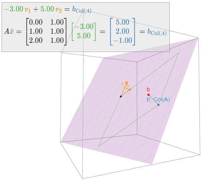
This solution minimizes the distance from \(A\hat x\) to \(b\text{,}\) i.e., the sum of the squares of the entries of \(b-A\hat x = b-b_{\text{Col}(A)} = b_{\text{Col}(A)^\perp}\). In this case, we have
\[||b-A\hat{x}||=\left|\left|\left(\begin{array}{c}6\\0\\0\end{array}\right)-\left(\begin{array}{c}5\\2\\-1\end{array}\right)\right|\right|=\left|\left|\left(\begin{array}{c}1\\-2\\1\end{array}\right)\right|\right|=\sqrt{1^2+(-2)^2+1^2}=\sqrt{6}.\nonumber\]
Therefore, \(b_{\text{Col}(A)} = A\hat x\) is \(\sqrt 6\) units from \(b.\)
In the following picture, \(v_1,v_2\) are the columns of \(A\text{:}\)
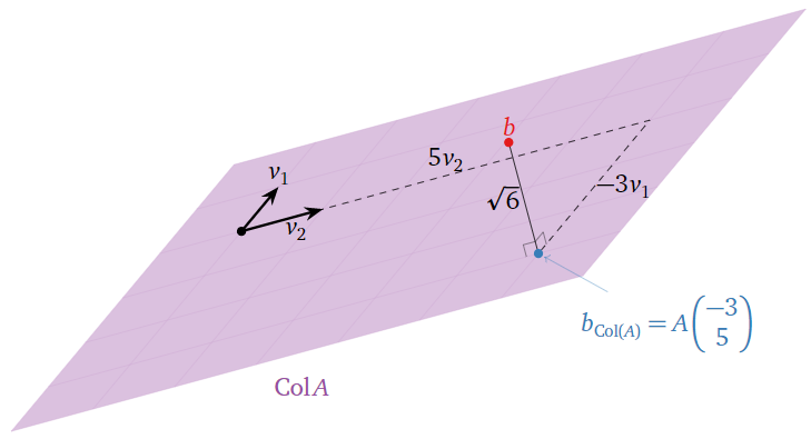
Figure \(\PageIndex{4}\)
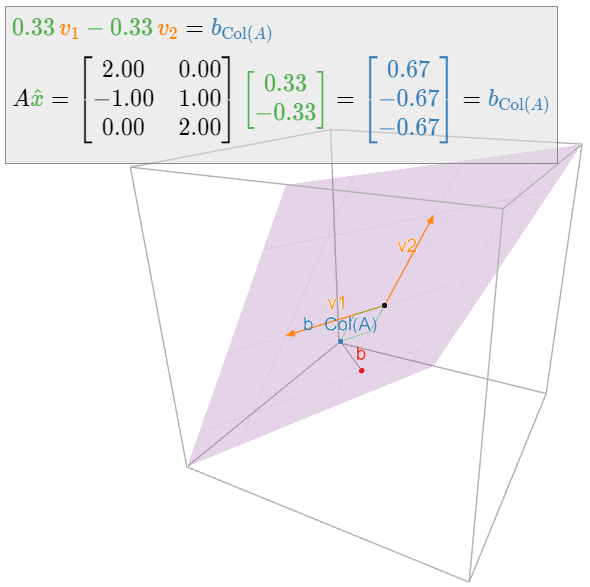
Find the least-squares solutions of \(Ax=b\) where:
\[ A = \left(\begin{array}{cc}2&0\\-1&1\\0&2\end{array}\right) \qquad b = \left(\begin{array}{c}1\\0\\-1\end{array}\right). \nonumber \]
Solution
We have
\[ A^T A = \left(\begin{array}{ccc}2&-1&0\\0&1&2\end{array}\right)\left(\begin{array}{cc}2&0\\-1&1\\0&2\end{array}\right) = \left(\begin{array}{cc}5&-1\\-1&5\end{array}\right) \nonumber \]
and
\[ A^T b = \left(\begin{array}{ccc}2&-1&0\\0&1&2\end{array}\right)\left(\begin{array}{c}1\\0\\-1\end{array}\right) = \left(\begin{array}{c}2\\-2\end{array}\right). \nonumber \]
We form an augmented matrix and row reduce:
\[ \left(\begin{array}{cc|c}5&-1&2\\-1&5&-2\end{array}\right)\xrightarrow{\text{RREF}}\left(\begin{array}{cc|c}1&0&1/3\\0&1&-1/3\end{array}\right). \nonumber \]
Therefore, the only least-squares solution is \(\hat x = \frac 13{1\choose -1}.\)
The reader may have noticed that we have been careful to say “the least-squares solutions” in the plural, and “a least-squares solution” using the indefinite article. This is because a least-squares solution need not be unique: indeed, if the columns of \(A\) are linearly dependent, then \(Ax=b_{\text{Col}(A)}\) has infinitely many solutions. The following theorem, which gives equivalent criteria for uniqueness, is an analogue of Corollary 6.3.1 in Section 6.3.
Let \(A\) be an \(m\times n\) matrix and let \(b\) be a vector in \(\mathbb{R}^m \). The following are equivalent:
- \(Ax=b\) has a unique least-squares solution.
- The columns of \(A\) are linearly independent.
- \(A^TA\) is invertible.
In this case, the least-squares solution is
\[ \hat x = (A^TA)^{-1} A^Tb. \nonumber \]
- Proof
-
The set of least-squares solutions of \(Ax=b\) is the solution set of the consistent equation \(A^TAx=A^Tb\text{,}\) which is a translate of the solution set of the homogeneous equation \(A^TAx=0\). Since \(A^TA\) is a square matrix, the equivalence of 1 and 3 follows from Theorem 5.1.1 in Section 5.1. The set of least squares-solutions is also the solution set of the consistent equation \(Ax = b_{\text{Col}(A)}\text{,}\) which has a unique solution if and only if the columns of \(A\) are linearly independent by Recipe: Checking Linear Independence in Section 2.5.
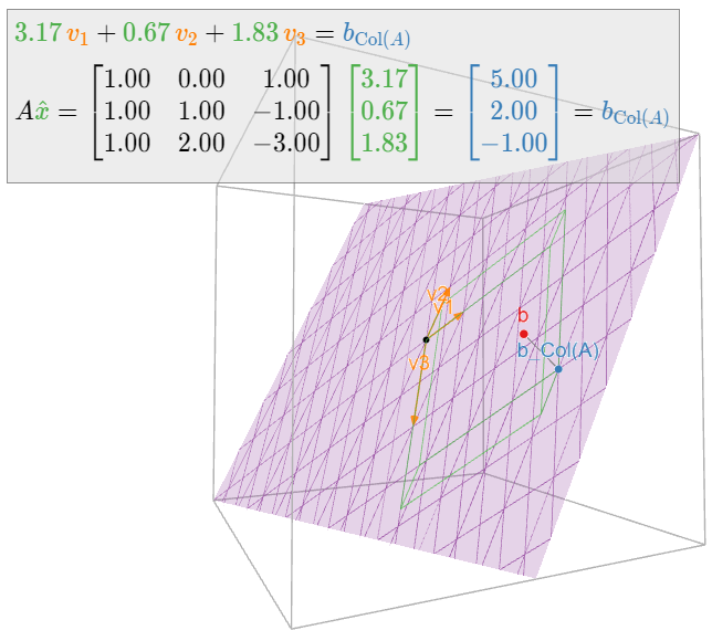
Find the least-squares solutions of \(Ax=b\) where:
\[ A = \left(\begin{array}{ccc}1&0&1\\1&1&-1\\1&2&-3\end{array}\right) \qquad b = \left(\begin{array}{c}6\\0\\0\end{array}\right). \nonumber \]
Solution
We have
\[ A^TA = \left(\begin{array}{ccc}3&3&-3\\3&5&-7\\-3&-7&11\end{array}\right) \qquad A^Tb = \left(\begin{array}{c}6\\0\\6\end{array}\right). \nonumber \]
We form an augmented matrix and row reduce:
\[ \left(\begin{array}{ccc|c}3&3&-3&6\\3&5&-7&0\\-3&-7&11&6\end{array}\right)\xrightarrow{\text{RREF}}\left(\begin{array}{ccc|c}1&0&1&5\\0&1&-2&-3\\0&0&0&0\end{array}\right). \nonumber \]
The free variable is \(x_3\text{,}\) so the solution set is
\[\left\{\begin{array}{rrrrr}x_1 &=& -x_3 &+& 5\\ x_2 &=& 2x_3 &-& 3\\ x_3 &=& x_3&{}&{}\end{array}\right. \quad\xrightarrow[\text{vector form}]{\text{parametric}}\quad \hat{x}=\left(\begin{array}{c}x_1\\x_2\\x_3\end{array}\right)=x_3\left(\begin{array}{c}-1\\2\\1\end{array}\right)+\left(\begin{array}{c}5\\-3\\0\end{array}\right).\nonumber\]
For example, taking \(x_3 = 0\) and \(x_3=1\) gives the least-squares solutions
\[ \hat x = \left(\begin{array}{c}5\\-3\\0\end{array}\right)\quad\text{and}\quad \hat x =\left(\begin{array}{c}4\\-1\\1\end{array}\right). \nonumber \]
Geometrically, we see that the columns \(v_1,v_2,v_3\) of \(A\) are coplanar:
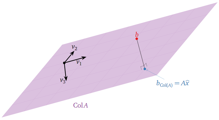
Figure \(\PageIndex{7}\)
Therefore, there are many ways of writing \(b_{\text{Col}(A)}\) as a linear combination of \(v_1,v_2,v_3\).
As usual, calculations involving projections become easier in the presence of an orthogonal set. Indeed, if \(A\) is an \(m\times n\) matrix with orthogonal columns \(u_1,u_2,\ldots,u_m\text{,}\) then we can use the Theorem 6.4.1 in Section 6.4 to write
\[ b_{\text{Col}(A)} = \frac{b\cdot u_1}{u_1\cdot u_1}\,u_1 + \frac{b\cdot u_2}{u_2\cdot u_2}\,u_2 + \cdots + \frac{b\cdot u_m}{u_m\cdot u_m}\,u_m = A\left(\begin{array}{c}(b\cdot u_1)/(u_1\cdot u_1) \\ (b\cdot u_2)/(u_2\cdot u_2) \\ \vdots \\ (b\cdot u_m)/(u_m\cdot u_m)\end{array}\right). \nonumber \]
Note that the least-squares solution is unique in this case, since an orthogonal set is linearly independent, Fact 6.4.1 in Section 6.4.
Let \(A\) be an \(m\times n\) matrix with orthogonal columns \(u_1,u_2,\ldots,u_m\text{,}\) and let \(b\) be a vector in \(\mathbb{R}^n \). Then the least-squares solution of \(Ax=b\) is the vector
\[ \hat x = \left(\frac{b\cdot u_1}{u_1\cdot u_1},\; \frac{b\cdot u_2}{u_2\cdot u_2},\; \ldots,\; \frac{b\cdot u_m}{u_m\cdot u_m} \right). \nonumber \]
This formula is particularly useful in the sciences, as matrices with orthogonal columns often arise in nature.
Find the least-squares solution of \(Ax=b\) where:
\[ A = \left(\begin{array}{ccc}1&0&1\\0&1&1\\-1&0&1\\0&-1&1\end{array}\right) \qquad b = \left(\begin{array}{c}0\\1\\3\\4\end{array}\right). \nonumber \]
Solution
Let \(u_1,u_2,u_3\) be the columns of \(A\). These form an orthogonal set, so
\[ \hat x = \left(\frac{b\cdot u_1}{u_1\cdot u_1},\; \frac{b\cdot u_2}{u_2\cdot u_2},\; \frac{b\cdot u_3}{u_3\cdot u_3} \right) = \left(\frac{-3}{2},\;\frac{-3}{2},\;\frac{8}{4}\right) = \left(-\frac32,\;-\frac32,\;2\right). \nonumber \]
Compare Example 6.4.8 in Section 6.4.
Best-Fit Problems
In this subsection we give an application of the method of least squares to data modeling. We begin with a basic example.
Suppose that we have measured three data points
\[ (0,6),\quad (1,0),\quad (2,0), \nonumber \]
and that our model for these data asserts that the points should lie on a line. Of course, these three points do not actually lie on a single line, but this could be due to errors in our measurement. How do we predict which line they are supposed to lie on?
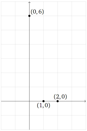
Figure \(\PageIndex{9}\)
The general equation for a (non-vertical) line is
\[ y = Mx + B. \nonumber \]
If our three data points were to lie on this line, then the following equations would be satisfied:
\[\begin{align} 6&=M\cdot 0+B\nonumber \\ 0&=M\cdot 1+B\label{eq:1} \\ 0&=M\cdot 2+B.\nonumber\end{align}\]
In order to find the best-fit line, we try to solve the above equations in the unknowns \(M\) and \(B\). As the three points do not actually lie on a line, there is no actual solution, so instead we compute a least-squares solution.
Putting our linear equations into matrix form, we are trying to solve \(Ax=b\) for
\[ A = \left(\begin{array}{cc}0&1\\1&1\\2&1\end{array}\right) \qquad x = \left(\begin{array}{c}M\\B\end{array}\right)\qquad b = \left(\begin{array}{c}6\\0\\0\end{array}\right). \nonumber \]
We solved this least-squares problem in Example \(\PageIndex{1}\): the only least-squares solution to \(Ax=b\) is \(\hat x = {M\choose B} = {-3\choose 5}\text{,}\) so the best-fit line is
\[ y = -3x + 5. \nonumber \]
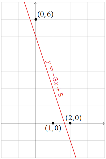
Figure \(\PageIndex{10}\)
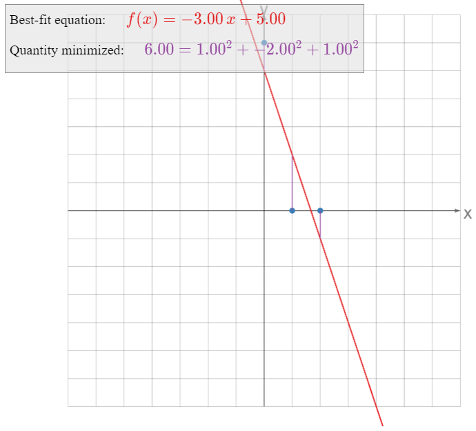
What exactly is the line \(y= f(x) = -3x+5\) minimizing? The least-squares solution \(\hat x\) minimizes the sum of the squares of the entries of the vector \(b-A\hat x\). The vector \(b\) is the left-hand side of \(\eqref{eq:1}\), and
\[ A\left(\begin{array}{c}-3\\5\end{array}\right) = \left(\begin{array}{c}-3(0)+5\\-3(1)+5\\-3(2)+5\end{array}\right) = \left(\begin{array}{c}f(0)\\f(1)\\f(2)\end{array}\right). \nonumber \]
In other words, \(A\hat x\) is the vector whose entries are the \(y\)-coordinates of the graph of the line at the values of \(x\) we specified in our data points, and \(b\) is the vector whose entries are the \(y\)-coordinates of those data points. The difference \(b-A\hat x\) is the vertical distance of the graph from the data points:
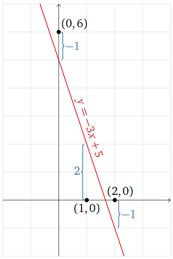
Figure \(\PageIndex{11}\)
\[\color{blue}{b-A\hat{x}=\left(\begin{array}{c}6\\0\\0\end{array}\right)-A\left(\begin{array}{c}-3\\5\end{array}\right)=\left(\begin{array}{c}-1\\2\\-1\end{array}\right)}\nonumber\]
The best-fit line minimizes the sum of the squares of these vertical distances.
Find the parabola that best approximates the data points
\[ (-1,\,1/2),\quad(1,\,-1),\quad(2,\,-1/2),\quad(3,\,2). \nonumber \]
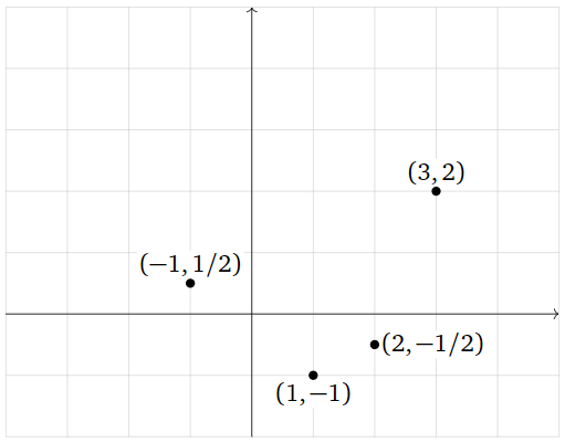
Figure \(\PageIndex{13}\)
What quantity is being minimized?
Solution
The general equation for a parabola is
\[ y = Bx^2 + Cx + D. \nonumber \]
If the four points were to lie on this parabola, then the following equations would be satisfied:
\[\begin{align} \frac{1}{2}&=B(-1)^2+C(-1)+D\nonumber \\ -1&=B(1)^2+C(1)+D\nonumber \\ -\frac{1}{2}&=B(2)^2+C(2)+D\label{eq:2} \\ 2&=B(3)^2+C(3)+D.\nonumber\end{align}\]
We treat this as a system of equations in the unknowns \(B,C,D\). In matrix form, we can write this as \(Ax=b\) for
\[ A = \left(\begin{array}{ccc}1&-1&1\\1&1&1\\4&2&1\\9&3&1\end{array}\right) \qquad x = \left(\begin{array}{c}B\\C\\D\end{array}\right) \qquad b = \left(\begin{array}{c}1/2 \\ -1\\-1/2 \\ 2\end{array}\right). \nonumber \]
We find a least-squares solution by multiplying both sides by the transpose:
\[ A^TA = \left(\begin{array}{ccc}99&35&15\\35&15&5\\15&5&4\end{array}\right) \qquad A^Tb = \left(\begin{array}{c}31/2\\7/2\\1\end{array}\right), \nonumber \]
then forming an augmented matrix and row reducing:
\[ \left(\begin{array}{ccc|c}99&35&15&31/2 \\ 35&15&5&7/2 \\ 15&5&4&1\end{array}\right)\xrightarrow{\text{RREF}}\left(\begin{array}{ccc|c}1&0&0&53/88 \\ 0&1&0&-379/440 \\ 0&0&1&-41/44\end{array}\right) \implies \hat x = \left(\begin{array}{c}53/88 \\ -379/440 \\ -41/44 \end{array}\right). \nonumber \]
The best-fit parabola is
\[ y = \frac{53}{88}x^2 - \frac{379}{440}x - \frac{41}{44}. \nonumber \]
Multiplying through by \(88\text{,}\) we can write this as
\[ 88y = 53x^2 - \frac{379}{5}x - 82. \nonumber \]
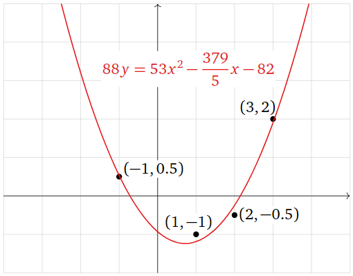
Figure \(\PageIndex{14}\)
Now we consider what exactly the parabola \(y = f(x)\) is minimizing. The least-squares solution \(\hat x\) minimizes the sum of the squares of the entries of the vector \(b-A\hat x\). The vector \(b\) is the left-hand side of \(\eqref{eq:2}\), and
\[A\hat{x}=\left(\begin{array}{c} \frac{53}{88}(-1)^2-\frac{379}{440}(-1)-\frac{41}{44} \\ \frac{53}{88}(1)^2-\frac{379}{440}(1)-\frac{41}{44} \\ \frac{53}{88}(2)^2-\frac{379}{440}(2)-\frac{41}{44} \\ \frac{53}{88}(3)^2-\frac{379}{440}(3)-\frac{41}{44}\end{array}\right)=\left(\begin{array}{c}f(-1) \\ f(1) \\ f(2) \\ f(3)\end{array}\right).\nonumber\]
In other words, \(A\hat x\) is the vector whose entries are the \(y\)-coordinates of the graph of the parabola at the values of \(x\) we specified in our data points, and \(b\) is the vector whose entries are the \(y\)-coordinates of those data points. The difference \(b-A\hat x\) is the vertical distance of the graph from the data points:
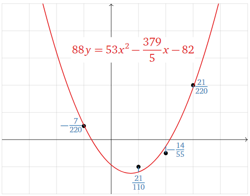
Figure \(\PageIndex{15}\)
\[\color{blue}{b-A\hat{x}=\left(\begin{array}{c}1/2 \\ -1 \\ -1/2 \\ 2\end{array}\right)-A\left(\begin{array}{c}53/88 \\ -379/440 \\ -41/44\end{array}\right)=\left(\begin{array}{c}-7/220 \\ 21/110 \\ -14/55 \\ 21/220\end{array}\right)}\nonumber\]
The best-fit parabola minimizes the sum of the squares of these vertical distances.
Find the linear function \(f(x,y)\) that best approximates the following data:
\[ \begin{array}{r|r|c} x & y & f(x,y) \\\hline 1 & 0 & 0 \\ 0 & 1 & 1 \\ -1 & 0 & 3 \\ 0 & -1 & 4 \end{array} \nonumber \]
What quantity is being minimized?
Solution
The general equation for a linear function in two variables is
\[ f(x,y) = Bx + Cy + D. \nonumber \]
We want to solve the following system of equations in the unknowns \(B,C,D\text{:}\)
\[\begin{align} B(1)+C(0)+D&=0 \nonumber \\ B(0)+C(1)+D&=1 \nonumber \\ B(-1)+C(0)+D&=3\label{eq:3} \\ B(0)+C(-1)+D&=4\nonumber\end{align}\]
In matrix form, we can write this as \(Ax=b\) for
\[ A = \left(\begin{array}{ccc}1&0&1\\0&1&1\\-1&0&1\\0&-1&1\end{array}\right) \qquad x = \left(\begin{array}{c}B\\C\\D\end{array}\right) \qquad b = \left(\begin{array}{c}0\\1\\3\\4\end{array}\right). \nonumber \]
We observe that the columns \(u_1,u_2,u_3\) of \(A\) are orthogonal, so we can use Recipe 2: Compute a Least-Squares Solution:
\[ \hat x = \left(\frac{b\cdot u_1}{u_1\cdot u_1},\; \frac{b\cdot u_2}{u_2\cdot u_2},\; \frac{b\cdot u_3}{u_3\cdot u_3} \right) = \left(\frac{-3}{2},\;\frac{-3}{2},\;\frac{8}{4}\right) = \left(-\frac32,\;-\frac32,\;2\right). \nonumber \] We find a least-squares solution by multiplying both sides by the transpose:
\[ A^TA = \left(\begin{array}{ccc}2&0&0\\0&2&0\\0&0&4\end{array}\right) \qquad A^Tb = \left(\begin{array}{c}-3\\-3\\8\end{array}\right). \nonumber \] The matrix \(A^TA\) is diagonal (do you see why that happened?), so it is easy to solve the equation \(A^TAx = A^Tb\text{:}\)
\[ \left(\begin{array}{cccc}2&0&0&-3 \\ 0&2&0&-3 \\ 0&0&4&8\end{array}\right) \xrightarrow{\text{RREF}} \left(\begin{array}{cccc}1&0&0&-3/2 \\ 0&1&0&-3/2 \\ 0&0&1&2\end{array}\right) \implies \hat x = \left(\begin{array}{c}-3/2 \\ -3/2 \\ 2\end{array}\right). \nonumber \] Therefore, the best-fit linear equation is
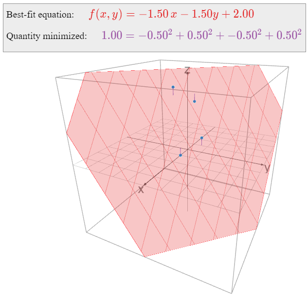
\[ f(x,y) = -\frac 32x - \frac32y + 2. \nonumber \]
Here is a picture of the graph of \(f(x,y)\text{:}\)
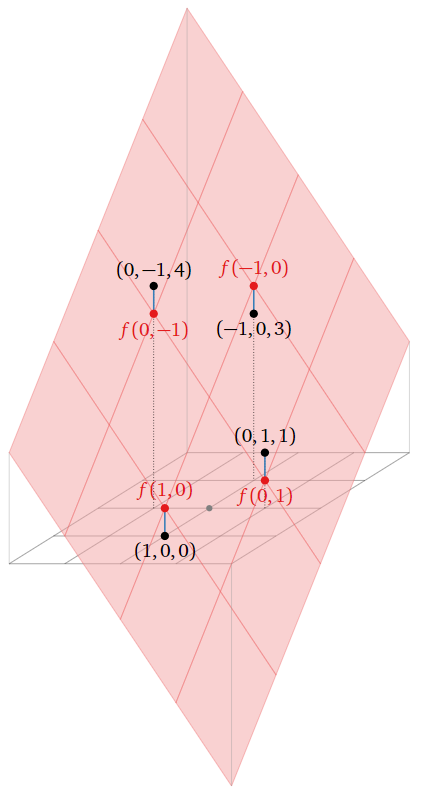
Figure \(\PageIndex{17}\)
Now we consider what quantity is being minimized by the function \(f(x,y)\). The least-squares solution \(\hat x\) minimizes the sum of the squares of the entries of the vector \(b-A\hat x\). The vector \(b\) is the right-hand side of \(\eqref{eq:3}\), and
\[A\hat{x}=\left(\begin{array}{rrrrr}-\frac32(1) &-& \frac32(0) &+& 2\\ -\frac32(0) &-& \frac32(1) &+& 2\\ -\frac32(-1) &-& \frac32(0) &+& 2\\ -\frac32(0) &-& \frac32(-1) &+& 2\end{array}\right)=\left(\begin{array}{c}f(1,0) \\ f(0,1) \\ f(-1,0) \\ f(0,-1)\end{array}\right).\nonumber\]
In other words, \(A\hat x\) is the vector whose entries are the values of \(f\) evaluated on the points \((x,y)\) we specified in our data table, and \(b\) is the vector whose entries are the desired values of \(f\) evaluated at those points. The difference \(b-A\hat x\) is the vertical distance of the graph from the data points, as indicated in the above picture. The best-fit linear function minimizes the sum of these vertical distances.
All of the above examples have the following form: some number of data points \((x,y)\) are specified, and we want to find a function
\[ y = B_1g_1(x) + B_2g_2(x) + \cdots + B_mg_m(x) \nonumber \]
that best approximates these points, where \(g_1,g_2,\ldots,g_m\) are fixed functions of \(x\). Indeed, in the best-fit line example we had \(g_1(x)=x\) and \(g_2(x)=1\text{;}\) in the best-fit parabola example we had \(g_1(x)=x^2\text{,}\) \(g_2(x)=x\text{,}\) and \(g_3(x)=1\text{;}\) and in the best-fit linear function example we had \(g_1(x_1,x_2)=x_1\text{,}\) \(g_2(x_1,x_2)=x_2\text{,}\) and \(g_3(x_1,x_2)=1\) (in this example we take \(x\) to be a vector with two entries). We evaluate the above equation on the given data points to obtain a system of linear equations in the unknowns \(B_1,B_2,\ldots,B_m\)—once we evaluate the \(g_i\text{,}\) they just become numbers, so it does not matter what they are—and we find the least-squares solution. The resulting best-fit function minimizes the sum of the squares of the vertical distances from the graph of \(y = f(x)\) to our original data points.
To emphasize that the nature of the functions \(g_i\) really is irrelevant, consider the following example.
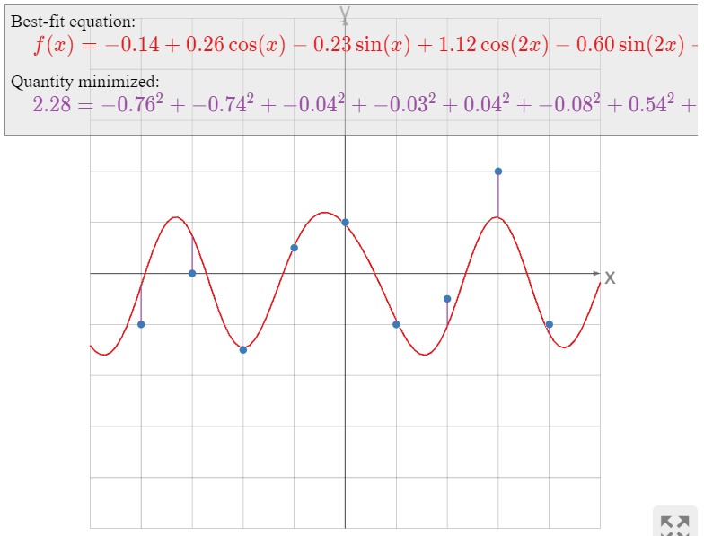
What is the best-fit function of the form
\[ y=B+C\cos(x)+D\sin(x)+E\cos(2x)+F\sin(2x)+G\cos(3x)+H\sin(3x) \nonumber \]
passing through the points
\[ \left(\begin{array}{c}-4\\ -1\end{array}\right),\; \left(\begin{array}{c}-3\\ 0\end{array}\right),\; \left(\begin{array}{c}-2\\ -1.5\end{array}\right),\; \left(\begin{array}{c}-1\\ .5\end{array}\right),\; \left(\begin{array}{c}0\\1\end{array}\right),\; \left(\begin{array}{c}1\\-1\end{array}\right),\; \left(\begin{array}{c}2\\-.5\end{array}\right),\; \left(\begin{array}{c}3\\2\end{array}\right),\; \left(\begin{array}{c}4 \\-1\end{array}\right)? \nonumber \]
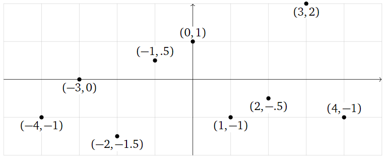
Figure \(\PageIndex{19}\)
Solution
We want to solve the system of equations
\[\begin{array}{rrrrrrrrrrrrrrr} -1 &=& B &+& C\cos(-4) &+& D\sin(-4) &+& E\cos(-8) &+& F\sin(-8) &+& G\cos(-12) &+& H\sin(-12)\\ 0 &=& B &+& C\cos(-3) &+& D\sin(-3) &+& E\cos(-6) &+& F\sin(-6) &+& G\cos(-9) &+& H\sin(-9)\\ -1.5 &=& B &+& C\cos(-2) &+& D\sin(-2) &+& E\cos(-4) &+& F\sin(-4) &+& G\cos(-6) &+& H\sin(-6) \\ 0.5 &=& B &+& C\cos(-1) &+& D\sin(-1) &+& E\cos(-2) &+& F\sin(-2) &+& G\cos(-3) &+& H\sin(-3)\\ 1 &=& B &+& C\cos(0) &+& D\sin(0) &+& E\cos(0) &+& F\sin(0) &+& G\cos(0) &+& H\sin(0)\\ -1 &=& B &+& C\cos(1) &+& D\sin(1) &+& E\cos(2) &+& F\sin(2) &+& G\cos(3) &+& H\sin(3)\\ -0.5 &=& B &+& C\cos(2) &+& D\sin(2) &+& E\cos(4) &+& F\sin(4) &+& G\cos(6) &+& H\sin(6)\\ 2 &=& B &+& C\cos(3) &+& D\sin(3) &+& E\cos(6) &+& F\sin(6) &+& G\cos(9) &+& H\sin(9)\\ -1 &=& B &+& C\cos(4) &+& D\sin(4) &+& E\cos(8) &+& F\sin(8) &+& G\cos(12) &+& H\sin(12).\end{array}\nonumber\]
All of the terms in these equations are numbers, except for the unknowns \(B,C,D,E,F,G,H\text{:}\)
\[\begin{array}{rrrrrrrrrrrrrrr} -1 &=& B &-& 0.6536C &+& 0.7568D &-& 0.1455E &-& 0.9894F &+& 0.8439G &+& 0.5366H\\ 0 &=& B &-& 0.9900C &-& 0.1411D &+& 0.9602E &+& 0.2794F &-& 0.9111G &-& 0.4121H\\ -1.5 &=& B &-& 0.4161C &-& 0.9093D &-& 0.6536E &+& 0.7568F &+& 0.9602G &+& 0.2794H\\ 0.5 &=& B &+& 0.5403C &-& 0.8415D &-& 0.4161E &-& 0.9093F &-& 0.9900G &-& 0.1411H\\ 1&=&B&+&C&{}&{}&+&E&{}&{}&+&G&{}&{}\\ -1 &=& B &+& 0.5403C &+& 0.8415D &-& 0.4161E &+& 0.9093F &-& 0.9900G &+& 0.1411H\\ -0.5 &=& B &-& 0.4161C &+& 0.9093D &-& 0.6536E &-& 0.7568F &+& 0.9602G &-& 0.2794H\\ 2 &=& B &-& 0.9900C &+& 0.1411D &+& 0.9602E &-& 0.2794F &-& 0.9111G &+& 0.4121H\\ -1 &=& B &-& 0.6536C &-& 0.7568D &-& 0.1455E &+& 0.9894F &+& 0.8439G &-& 0.5366H.\end{array}\nonumber\]
Hence we want to solve the least-squares problem
\[\left(\begin{array}{rrrrrrr} 1 &-0.6536& 0.7568& -0.1455& -0.9894& 0.8439 &0.5366\\ 1& -0.9900& -0.1411 &0.9602 &0.2794& -0.9111& -0.4121\\ 1& -0.4161& -0.9093& -0.6536& 0.7568& 0.9602& 0.2794\\ 1& 0.5403& -0.8415 &-0.4161& -0.9093& -0.9900 &-0.1411\\ 1& 1& 0& 1& 0& 1& 0\\ 1& 0.5403& 0.8415& -0.4161& 0.9093& -0.9900 &0.1411\\ 1& -0.4161& 0.9093& -0.6536& -0.7568& 0.9602& -0.2794\\ 1& -0.9900 &0.1411 &0.9602& -0.2794& -0.9111& 0.4121\\ 1& -0.6536& -0.7568& -0.1455& 0.9894 &0.8439 &-0.5366\end{array}\right)\left(\begin{array}{c}B\\C\\D\\E\\F\\G\\H\end{array}\right)=\left(\begin{array}{c}-1\\0\\-1.5\\0.5\\1\\-1\\-0.5\\2\\-1\end{array}\right).\nonumber\]
We find the least-squares solution with the aid of a computer:
\[\hat{x}\approx\left(\begin{array}{c} -0.1435 \\0.2611 \\-0.2337\\ 1.116\\ -0.5997\\ -0.2767 \\0.1076\end{array}\right).\nonumber\]
Therefore, the best-fit function is
\[ \begin{split} y \amp\approx -0.1435 + 0.2611\cos(x) -0.2337\sin(x) + 1.116\cos(2x) -0.5997\sin(2x) \\ \amp\qquad\qquad -0.2767\cos(3x) + 0.1076\sin(3x). \end{split} \nonumber \]
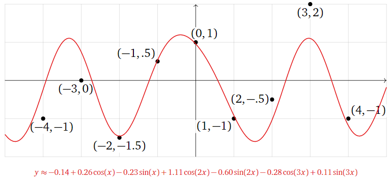
Figure \(\PageIndex{20}\)
As in the previous examples, the best-fit function minimizes the sum of the squares of the vertical distances from the graph of \(y = f(x)\) to the data points.
The next example has a somewhat different flavor from the previous ones.
Find the best-fit ellipse through the points
\[ (0,2),\, (2,1),\, (1,-1),\, (-1,-2),\, (-3,1),\, (-1,-1). \nonumber \]
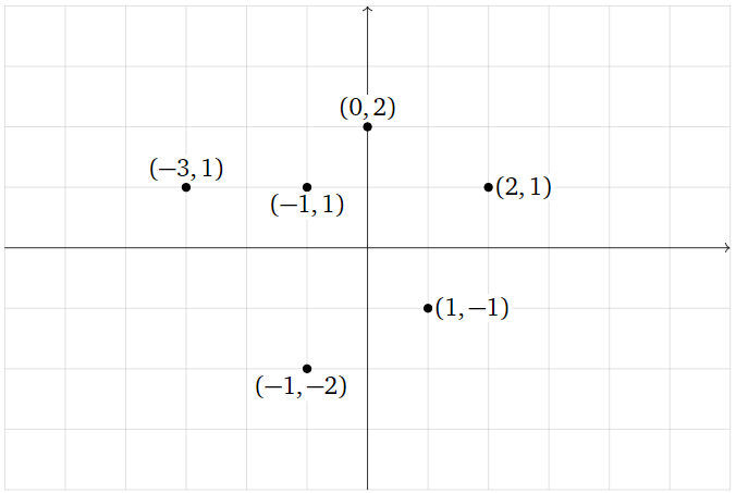
Figure \(\PageIndex{22}\)
What quantity is being minimized?
Solution
The general equation for an ellipse (actually, for a nondegenerate conic section) is
\[ x^2 + By^2 + Cxy + Dx + Ey + F = 0. \nonumber \]
This is an implicit equation: the ellipse is the set of all solutions of the equation, just like the unit circle is the set of solutions of \(x^2+y^2=1.\) To say that our data points lie on the ellipse means that the above equation is satisfied for the given values of \(x\) and \(y\text{:}\)
\[\label{eq:4} \begin{array}{rrrrrrrrrrrrl} (0)^2 &+& B(2)^2 &+& C(0)(2)&+& D(0) &+& E(2)&+& F&=& 0 \\ (2)^2 &+& B(1)^2 &+& C(2)(1)&+& D(2)&+&E(1)&+&F&=& 0 \\ (1)^2&+& B(-1)^2&+&C(1)(-1)&+&D(1)&+&E(-1)&+&F&=&0 \\ (-1)^2&+&B(-2)^2&+&C(-1)(2)&+&D(-1)&+&E(-2)&+&F&=&0 \\ (-3)^2&+&B(1)^2&+&C(-3)(1)&+&D(-3)&+&E(1)&+&F&=&0 \\ (-1)^2&+&B(-1)^2&+&C(-1)(-1)&+&D(-1)&+&E(-1)&+&F&=&0.\end{array}\]
To put this in matrix form, we move the constant terms to the right-hand side of the equals sign; then we can write this as \(Ax=b\) for
\[A=\left(\begin{array}{ccccc}4&0&0&2&1\\1&2&2&1&1\\1&-1&1&-1&1 \\ 4&2&-1&-2&1 \\ 1&-3&-3&1&1 \\ 1&1&-1&-1&1\end{array}\right)\quad x=\left(\begin{array}{c}B\\C\\D\\E\\F\end{array}\right)\quad b=\left(\begin{array}{c}0\\-4\\-1\\-1\\-9\\-1\end{array}\right).\nonumber\]
We compute
\[ A^TA = \left(\begin{array}{ccccc}36&7&-5&0&12 \\ 7&19&9&-5&1 \\ -5&9&16&1&-2 \\ 0&-5&1&12&0 \\ 12&1&-2&0&6\end{array}\right) \qquad A^T b = \left(\begin{array}{c}-19\\17\\20\\-9\\-16\end{array}\right). \nonumber \]
We form an augmented matrix and row reduce:
\[\left(\begin{array}{ccccc|c} 36 &7& -5& 0& 12& -19\\ 7& 19& 9& -5& 1& 17\\ -5& 9& 16& 1& -2& 20\\ 0& -5& 1 &12& 0& -9\\ 12& 1& -2& 0& 6& -16\end{array}\right)\xrightarrow{\text{RREF}}\left(\begin{array}{ccccc|c} 1& 0& 0& 0& 0& 405/266\\ 0& 1& 0& 0& 0& -89/133\\ 0& 0& 1& 0& 0& 201/133\\ 0& 0& 0& 1& 0& -123/266\\ 0& 0& 0& 0& 1& -687/133\end{array}\right).\nonumber\]
The least-squares solution is
\[\hat{x}=\left(\begin{array}{c}405/266\\ -89/133\\ 201/133\\ -123/266\\ -687/133\end{array}\right),\nonumber\]
so the best-fit ellipse is
\[ x^2 + \frac{405}{266} y^2 -\frac{89}{133} xy + \frac{201}{133}x - \frac{123}{266}y - \frac{687}{133} = 0. \nonumber \]
Multiplying through by \(266\text{,}\) we can write this as
\[ 266 x^2 + 405 y^2 - 178 xy + 402 x - 123 y - 1374 = 0. \nonumber \]
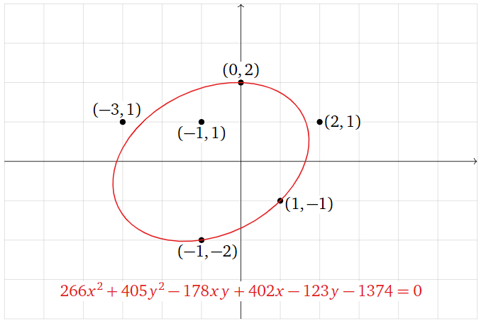
Figure \(\PageIndex{23}\)
Now we consider the question of what quantity is minimized by this ellipse. The least-squares solution \(\hat x\) minimizes the sum of the squares of the entries of the vector \(b-A\hat x\text{,}\) or equivalently, of \(A\hat x-b\). The vector \(-b\) contains the constant terms of the left-hand sides of \(\eqref{eq:4}\), and
\[A\hat{x}=\left(\begin{array}{rrrrrrrrr} \frac{405}{266}(2)^2 &-& \frac{89}{133}(0)(2)&+&\frac{201}{133}(0)&-&\frac{123}{266}(2)&-&\frac{687}{133} \\ \frac{405}{266}(1)^2&-& \frac{89}{133}(2)(1)&+&\frac{201}{133}(2)&-&\frac{123}{266}(1)&-&\frac{687}{133} \\ \frac{405}{266}(-1)^2 &-&\frac{89}{133}(1)(-1)&+&\frac{201}{133}(1)&-&\frac{123}{266}(-1)&-&\frac{687}{133} \\ \frac{405}{266}(-2)^2&-&\frac{89}{133}(-1)(-2)&+&\frac{201}{133}(-1)&-&\frac{123}{266}(-2)&-&\frac{687}{133} \\ \frac{405}{266}(1)^2&-&\frac{89}{133}(-3)(1)&+&\frac{201}{133}(-3)&-&\frac{123}{266}(1)&-&\frac{687}{133} \\ \frac{405}{266}(-1)^2&-&\frac{89}{133}(-1)(-1)&+&\frac{201}{133}(-1)&-&\frac{123}{266}(-1)&-&\frac{687}{133}\end{array}\right)\nonumber\]
contains the rest of the terms on the left-hand side of \(\eqref{eq:4}\). Therefore, the entries of \(A\hat x-b\) are the quantities obtained by evaluating the function
\[ f(x,y) = x^2 + \frac{405}{266} y^2 -\frac{89}{133} xy + \frac{201}{133}x - \frac{123}{266}y - \frac{687}{133} \nonumber \]
on the given data points.
If our data points actually lay on the ellipse defined by \(f(x,y)=0\text{,}\) then evaluating \(f(x,y)\) on our data points would always yield zero, so \(A\hat x-b\) would be the zero vector. This is not the case; instead, \(A\hat x-b\) contains the actual values of \(f(x,y)\) when evaluated on our data points. The quantity being minimized is the sum of the squares of these values:
\[ \begin{split} \amp\text{minimized} = \\ \amp\quad f(0,2)^2 + f(2,1)^2 + f(1,-1)^2 + f(-1,-2)^2 + f(-3,1)^2 + f(-1,-1)^2. \end{split} \nonumber \]
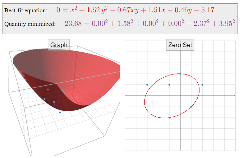
One way to visualize this is as follows. We can put this best-fit problem into the framework of Example \(\PageIndex{8}\) by asking to find an equation of the form
\[ f(x,y) = x^2 + By^2 + Cxy + Dx + Ey + F \nonumber \]
which best approximates the data table
\[ \begin{array}{r|r|c} x & y & f(x,y) \\\hline 0 & 2 & 0 \\ 2 & 1 & 0 \\ 1 & -1 & 0 \\ -1 & -2 & 0 \\ -3 & 1 & 0 \\ -1 & -1 & 0\rlap. \end{array} \nonumber \]
The resulting function minimizes the sum of the squares of the vertical distances from these data points \((0,2,0),\,(2,1,0),\,\ldots\text{,}\) which lie on the \(xy\)-plane, to the graph of \(f(x,y)\).
Gauss invented the method of least squares to find a best-fit ellipse: he correctly predicted the (elliptical) orbit of the asteroid Ceres as it passed behind the sun in 1801.