
3.4: Matrix Multiplication
- Page ID
- 70198

\( \newcommand{\vecs}[1]{\overset { \scriptstyle \rightharpoonup} {\mathbf{#1}} } \)
\( \newcommand{\vecd}[1]{\overset{-\!-\!\rightharpoonup}{\vphantom{a}\smash {#1}}} \)
\( \newcommand{\dsum}{\displaystyle\sum\limits} \)
\( \newcommand{\dint}{\displaystyle\int\limits} \)
\( \newcommand{\dlim}{\displaystyle\lim\limits} \)
\( \newcommand{\id}{\mathrm{id}}\) \( \newcommand{\Span}{\mathrm{span}}\)
( \newcommand{\kernel}{\mathrm{null}\,}\) \( \newcommand{\range}{\mathrm{range}\,}\)
\( \newcommand{\RealPart}{\mathrm{Re}}\) \( \newcommand{\ImaginaryPart}{\mathrm{Im}}\)
\( \newcommand{\Argument}{\mathrm{Arg}}\) \( \newcommand{\norm}[1]{\| #1 \|}\)
\( \newcommand{\inner}[2]{\langle #1, #2 \rangle}\)
\( \newcommand{\Span}{\mathrm{span}}\)
\( \newcommand{\id}{\mathrm{id}}\)
\( \newcommand{\Span}{\mathrm{span}}\)
\( \newcommand{\kernel}{\mathrm{null}\,}\)
\( \newcommand{\range}{\mathrm{range}\,}\)
\( \newcommand{\RealPart}{\mathrm{Re}}\)
\( \newcommand{\ImaginaryPart}{\mathrm{Im}}\)
\( \newcommand{\Argument}{\mathrm{Arg}}\)
\( \newcommand{\norm}[1]{\| #1 \|}\)
\( \newcommand{\inner}[2]{\langle #1, #2 \rangle}\)
\( \newcommand{\Span}{\mathrm{span}}\) \( \newcommand{\AA}{\unicode[.8,0]{x212B}}\)
\( \newcommand{\vectorA}[1]{\vec{#1}} % arrow\)
\( \newcommand{\vectorAt}[1]{\vec{\text{#1}}} % arrow\)
\( \newcommand{\vectorB}[1]{\overset { \scriptstyle \rightharpoonup} {\mathbf{#1}} } \)
\( \newcommand{\vectorC}[1]{\textbf{#1}} \)
\( \newcommand{\vectorD}[1]{\overrightarrow{#1}} \)
\( \newcommand{\vectorDt}[1]{\overrightarrow{\text{#1}}} \)
\( \newcommand{\vectE}[1]{\overset{-\!-\!\rightharpoonup}{\vphantom{a}\smash{\mathbf {#1}}}} \)
\( \newcommand{\vecs}[1]{\overset { \scriptstyle \rightharpoonup} {\mathbf{#1}} } \)
\(\newcommand{\longvect}{\overrightarrow}\)
\( \newcommand{\vecd}[1]{\overset{-\!-\!\rightharpoonup}{\vphantom{a}\smash {#1}}} \)
\(\newcommand{\avec}{\mathbf a}\) \(\newcommand{\bvec}{\mathbf b}\) \(\newcommand{\cvec}{\mathbf c}\) \(\newcommand{\dvec}{\mathbf d}\) \(\newcommand{\dtil}{\widetilde{\mathbf d}}\) \(\newcommand{\evec}{\mathbf e}\) \(\newcommand{\fvec}{\mathbf f}\) \(\newcommand{\nvec}{\mathbf n}\) \(\newcommand{\pvec}{\mathbf p}\) \(\newcommand{\qvec}{\mathbf q}\) \(\newcommand{\svec}{\mathbf s}\) \(\newcommand{\tvec}{\mathbf t}\) \(\newcommand{\uvec}{\mathbf u}\) \(\newcommand{\vvec}{\mathbf v}\) \(\newcommand{\wvec}{\mathbf w}\) \(\newcommand{\xvec}{\mathbf x}\) \(\newcommand{\yvec}{\mathbf y}\) \(\newcommand{\zvec}{\mathbf z}\) \(\newcommand{\rvec}{\mathbf r}\) \(\newcommand{\mvec}{\mathbf m}\) \(\newcommand{\zerovec}{\mathbf 0}\) \(\newcommand{\onevec}{\mathbf 1}\) \(\newcommand{\real}{\mathbb R}\) \(\newcommand{\twovec}[2]{\left[\begin{array}{r}#1 \\ #2 \end{array}\right]}\) \(\newcommand{\ctwovec}[2]{\left[\begin{array}{c}#1 \\ #2 \end{array}\right]}\) \(\newcommand{\threevec}[3]{\left[\begin{array}{r}#1 \\ #2 \\ #3 \end{array}\right]}\) \(\newcommand{\cthreevec}[3]{\left[\begin{array}{c}#1 \\ #2 \\ #3 \end{array}\right]}\) \(\newcommand{\fourvec}[4]{\left[\begin{array}{r}#1 \\ #2 \\ #3 \\ #4 \end{array}\right]}\) \(\newcommand{\cfourvec}[4]{\left[\begin{array}{c}#1 \\ #2 \\ #3 \\ #4 \end{array}\right]}\) \(\newcommand{\fivevec}[5]{\left[\begin{array}{r}#1 \\ #2 \\ #3 \\ #4 \\ #5 \\ \end{array}\right]}\) \(\newcommand{\cfivevec}[5]{\left[\begin{array}{c}#1 \\ #2 \\ #3 \\ #4 \\ #5 \\ \end{array}\right]}\) \(\newcommand{\mattwo}[4]{\left[\begin{array}{rr}#1 \amp #2 \\ #3 \amp #4 \\ \end{array}\right]}\) \(\newcommand{\laspan}[1]{\text{Span}\{#1\}}\) \(\newcommand{\bcal}{\cal B}\) \(\newcommand{\ccal}{\cal C}\) \(\newcommand{\scal}{\cal S}\) \(\newcommand{\wcal}{\cal W}\) \(\newcommand{\ecal}{\cal E}\) \(\newcommand{\coords}[2]{\left\{#1\right\}_{#2}}\) \(\newcommand{\gray}[1]{\color{gray}{#1}}\) \(\newcommand{\lgray}[1]{\color{lightgray}{#1}}\) \(\newcommand{\rank}{\operatorname{rank}}\) \(\newcommand{\row}{\text{Row}}\) \(\newcommand{\col}{\text{Col}}\) \(\renewcommand{\row}{\text{Row}}\) \(\newcommand{\nul}{\text{Nul}}\) \(\newcommand{\var}{\text{Var}}\) \(\newcommand{\corr}{\text{corr}}\) \(\newcommand{\len}[1]{\left|#1\right|}\) \(\newcommand{\bbar}{\overline{\bvec}}\) \(\newcommand{\bhat}{\widehat{\bvec}}\) \(\newcommand{\bperp}{\bvec^\perp}\) \(\newcommand{\xhat}{\widehat{\xvec}}\) \(\newcommand{\vhat}{\widehat{\vvec}}\) \(\newcommand{\uhat}{\widehat{\uvec}}\) \(\newcommand{\what}{\widehat{\wvec}}\) \(\newcommand{\Sighat}{\widehat{\Sigma}}\) \(\newcommand{\lt}{<}\) \(\newcommand{\gt}{>}\) \(\newcommand{\amp}{&}\) \(\definecolor{fillinmathshade}{gray}{0.9}\)- Understand compositions of transformations.
- Understand the relationship between matrix products and compositions of matrix transformations.
- Become comfortable doing basic algebra involving matrices.
- Recipe: matrix multiplication (two ways).
- Picture: composition of transformations.
- Vocabulary word: composition.
In this section, we study compositions of transformations. As we will see, composition is a way of chaining transformations together. The composition of matrix transformations corresponds to a notion of multiplying two matrices together. We also discuss addition and scalar multiplication of transformations and of matrices.
Composition of Linear Transformations
Composition means the same thing in linear algebra as it does in Calculus. Here is the definition.
Let \(T\colon\mathbb{R}^n \to\mathbb{R}^m \) and \(U\colon\mathbb{R}^p \to\mathbb{R}^n \) be transformations. Their composition is the transformation \(T\circ U\colon\mathbb{R}^p \to\mathbb{R}^m \) defined by
\[ (T\circ U)(x) = T(U(x)). \nonumber \]
Composing two transformations means chaining them together: \(T\circ U\) is the transformation that first applies \(U\text{,}\) then applies \(T\) (note the order of operations). More precisely, to evaluate \(T\circ U\) on an input vector \(x\text{,}\) first you evaluate \(U(x)\text{,}\) then you take this output vector of \(U\) and use it as an input vector of \(T\text{:}\) that is, \((T\circ U)(x) = T(U(x))\). Of course, this only makes sense when the outputs of \(U\) are valid inputs of \(T\text{,}\) that is, when the range of \(U\) is contained in the domain of \(T\).
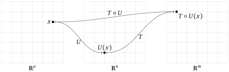
Figure \(\PageIndex{1}\)
Here is a picture of the composition \(T\circ U\) as a “machine” that first runs \(U\text{,}\) then takes its output and feeds it into \(T\text{;}\) there is a similar picture in Subsection Transformations in Section 3.1.
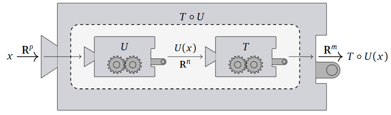
Figure \(\PageIndex{2}\)
- In order for \(T\circ U\) to be defined, the codomain of \(U\) must equal the domain of \(T\).
- The domain of \(T\circ U\) is the domain of \(U\).
- The codomain of \(T\circ U\) is the codomain of \(T\).
Define \(f\colon \mathbb{R} \to\mathbb{R} \) by \(f(x) = x^2\) and \(g\colon \mathbb{R} \to\mathbb{R} \) by \(g(x) = x^3\). The composition \(f\circ g\colon \mathbb{R} \to\mathbb{R} \) is the transformation defined by the rule
\[ f\circ g(x) = f(g(x)) = f(x^3) = (x^3)^2 = x^6. \nonumber \]
For instance, \(f\circ g(-2) = f(-8) = 64.\)
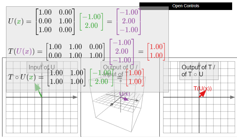
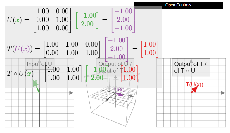
Define \(T\colon\mathbb{R}^3 \to\mathbb{R}^2 \) and \(U\colon\mathbb{R}^2 \to\mathbb{R}^3 \) by
\[T(x)=\left(\begin{array}{ccc}1&1&0\\0&1&1\end{array}\right)x\quad\text{and}\quad U(x)=\left(\begin{array}{cc}1&0\\0&1\\1&0\end{array}\right)x.\nonumber\]
Their composition is a transformation \(T\circ U\colon\mathbb{R}^2 \to\mathbb{R}^2 \text{;}\) it turns out to be the matrix transformation associated to the matrix \(\bigl(\begin{smallmatrix}1\amp1\\1\amp1\end{smallmatrix}\bigr)\).
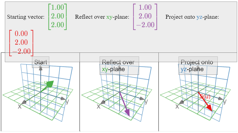
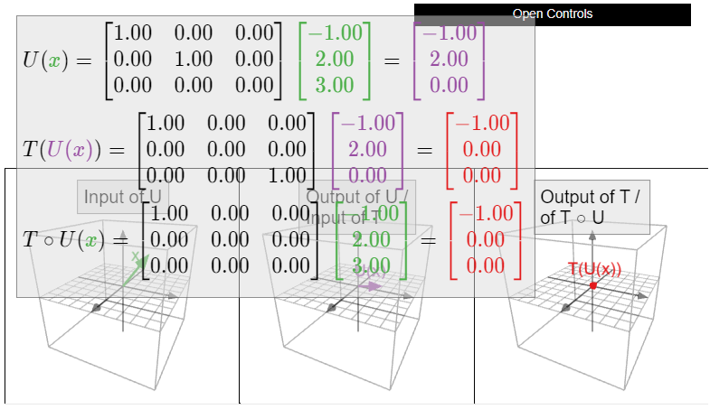
Let \(S\colon\mathbb{R}^3 \to\mathbb{R}^3 \) be the linear transformation that first reflects over the \(xy\)-plane and then projects onto the \(yz\)-plane, as in Example 3.3.10 in Section 3.3. The transformation \(S\) is the composition \(T\circ U\text{,}\) where \(U\colon\mathbb{R}^3 \to\mathbb{R}^3 \) is the transformation that reflects over the \(xy\)-plane, and \(T\colon\mathbb{R}^3 \to\mathbb{R}^3 \) is the transformation that projects onto the \(yz\)-plane.
Let \(S\colon\mathbb{R}^3 \to\mathbb{R}^3 \) be the linear transformation that first projects onto the \(xy\)-plane, and then projects onto the \(xz\)-plane. The transformation \(S\) is the composition \(T\circ U\text{,}\) where \(U\colon\mathbb{R}^3 \to\mathbb{R}^3 \) is the transformation that projects onto the \(xy\)-plane, and \(T\colon\mathbb{R}^3 \to\mathbb{R}^3 \) is the transformation that projects onto the \(xz\)-plane.
Recall from Definition 3.1.2 in Section 3.1 that the identity transformation is the transformation \(\operatorname{Id}_{\mathbb{R}^n }\colon\mathbb{R}^n \to\mathbb{R}^n \) defined by \(\operatorname{Id}_{\mathbb{R}^n }(x) = x\) for every vector \(x\).
Let \(S,T,U\) be transformations and let \(c\) be a scalar. Suppose that \(T\colon\mathbb{R}^n \to\mathbb{R}^m \text{,}\) and that in each of the following identities, the domains and the codomains are compatible when necessary for the composition to be defined. The following properties are easily verified:
\[\begin{align*} S\circ(T+U) \amp= S\circ T+S\circ U \amp (S + T)\circ U \amp= S\circ U + T\circ U \amp\\ c(T\circ U) \amp= (cT)\circ U \amp c(T\circ U) \amp= T\circ(cU) \rlap{\;\;\text{ if $T$ is linear}}\\ T\circ\operatorname{Id}_{\mathbb{R}^n } \amp= T \amp \operatorname{Id}_{\mathbb{R}^m }\circ T \amp= T\\ \amp \amp S\circ(T\circ U) \amp= (S\circ T)\circ U \amp \end{align*}\]
The final property is called associativity. Unwrapping both sides, it says:
\[ S\circ(T\circ U)(x) = S(T\circ U(x)) = S(T(U(x))) = S\circ T(U(x)) = (S\circ T)\circ U(x). \nonumber \]
In other words, both \(S\circ (T\circ U)\) and \((S\circ T)\circ U\) are the transformation defined by first applying \(U\text{,}\) then \(T\text{,}\) then \(S\).
Composition of transformations is not commutative in general. That is, in general, \(T\circ U\neq U\circ T\text{,}\) even when both compositions are defined.
Define \(f\colon \mathbb{R} \to\mathbb{R} \) by \(f(x) = x^2\) and \(g\colon \mathbb{R} \to\mathbb{R} \) by \(g(x) = e^x\). The composition \(f\circ g\colon \mathbb{R} \to\mathbb{R} \) is the transformation defined by the rule
\[ f\circ g(x) = f(g(x)) = f(e^x) = (e^x)^2 = e^{2x}. \nonumber \]
The composition \(g\circ f\colon \mathbb{R} \to\mathbb{R} \) is the transformation defined by the rule
\[ g\circ f(x) = g(f(x)) = g(x^2) = e^{x^2}. \nonumber \]
Note that \(e^{x^2}\neq e^{2x}\) in general; for instance, if \(x=1\) then \(e^{x^2} = e\) and \(e^{2x} = e^2\). Thus \(f \circ g\) is not equal to \(g \circ f\text{,}\) and we can already see with functions of one variable that composition of functions is not commutative.
Define matrix transformations \(T,U\colon\mathbb{R}^2 \to\mathbb{R}^2 \) by
\[ T(x) = \left(\begin{array}{cc}1&1\\0&1\end{array}\right)x \quad\text{and}\quad U(x) = \left(\begin{array}{cc}1&0\\1&1\end{array}\right)x. \nonumber \]
Geometrically, \(T\) is a shear in the \(x\)-direction, and \(U\) is a shear in the \(Y\)-direction. We evaluate
\[T\circ U\left(\begin{array}{c}1\\0\end{array}\right)=T\left(\begin{array}{c}1\\1\end{array}\right)=\left(\begin{array}{c}2\\1\end{array}\right)\nonumber\]
and
\[ U\circ T\left(\begin{array}{c}1\\0\end{array}\right) = U\left(\begin{array}{c}1\\0\end{array}\right) = \left(\begin{array}{c}1\\1\end{array}\right). \nonumber \]
Since \(T\circ U\) and \(U\circ T\) have different outputs for the input vector \(1\choose 0\text{,}\) they are different transformations. (See this Example \(\PageIndex{9}\).)
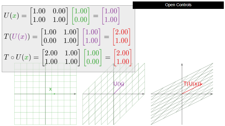
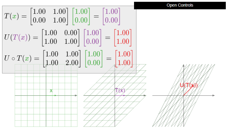
Figure \(\PageIndex{7}\): Illustration of the composition \(U\circ T\).
Matrix multiplication
In this subsection, we introduce a seemingly unrelated operation on matrices, namely, matrix multiplication. As we will see in the next subsection, matrix multiplication exactly corresponds to the composition of the corresponding linear transformations. First we need some terminology.
Let \(A\) be an \(m\times n\) matrix. We will generally write \(a_{ij}\) for the entry in the \(i\)th row and the \(j\)th column. It is called the \(i,j\) entry of the matrix.
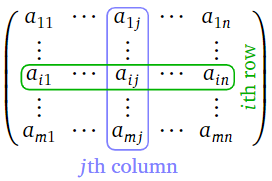
Figure \(\PageIndex{8}\)
Let \(A\) be an \(m\times n\) matrix and let \(B\) be an \(n\times p\) matrix. Denote the columns of \(B\) by \(v_1,v_2,\ldots,v_p\text{:}\)
\[B=\left(\begin{array}{cccc}|&|&\quad&| \\ v_1&v_2&\cdots &v_p \\ |&|&\quad&|\end{array}\right).\nonumber\]
The product \(AB\) is the \(m\times p\) matrix with columns \(Av_1,Av_2,\ldots,Av_p\text{:}\)
\[AB=\left(\begin{array}{cccc}|&|&\quad&| \\ Av_1&Av_2&\cdots &Av_p \\ |&|&\quad &|\end{array}\right).\nonumber\]
In other words, matrix multiplication is defined column-by-column, or “distributes over the columns of \(B\).”
\[\begin{aligned}\left(\begin{array}{ccc}1&1&0\\0&1&1\end{array}\right)\left(\begin{array}{cc}1&0\\0&1\\1&0\end{array}\right)&=\left(\left(\begin{array}{ccc}1&1&0\\0&1&1\end{array}\right)\left(\begin{array}{c}1\\0\\1\end{array}\right)\:\left(\begin{array}{ccc}1&1&0\\0&1&1\end{array}\right)\left(\begin{array}{c}0\\1\\0\end{array}\right)\right) \\ &=\left(\left(\begin{array}{c}1\\1\end{array}\right)\:\left(\begin{array}{c}1\\1\end{array}\right)\right)=\left(\begin{array}{cc}1&1\\1&1\end{array}\right)\end{aligned}\nonumber\]
In order for the vectors \(Av_1,Av_2,\ldots,Av_p\) to be defined, the numbers of rows of \(B\) has to equal the number of columns of \(A\).
- In order for \(AB\) to be defined, the number of rows of \(B\) has to equal the number of columns of \(A\).
- The product of an \(\color{blue}{m}\color{black}{\times}\color{Red}{n}\) matrix and an \(\color{red}{n}\color{black}{\times}\color{blue}{p}\) matrix is an \(\color{blue}{m}\color{black}{\times}\color{blue}{p}\) matrix.
If \(B\) has only one column, then \(AB\) also has one column. A matrix with one column is the same as a vector, so the definition of the matrix product generalizes the definition of the matrix-vector product from Definition 2.3.1 in Section 2.3.
If \(A\) is a square matrix, then we can multiply it by itself; we define its powers to be
\[ A^2 = AA \qquad A^3 = AAA \qquad \text{etc.} \nonumber \]
The row-column rule for matrix multiplication
Recall from Definition 2.3.3 in Section 2.3 that the product of a row vector and a column vector is the scalar
\[ \left(\begin{array}{cccc}a_1&a_2&\cdots &a_n\end{array}\right)\:\left(\begin{array}{c}x_1\\x_2\\ \vdots\\x_n\end{array}\right) = a_1x_1 + a_2x_2 + \cdots + a_nx_n. \nonumber \]
The following procedure for finding the matrix product is much better adapted to computations by hand; the previous Definition \(\PageIndex{3}\) is more suitable for proving theorems, such as this Theorem \(\PageIndex{1}\) below.
Let \(A\) be an \(m\times n\) matrix, let \(B\) be an \(n\times p\) matrix, and let \(C = AB\). Then the \(ij\) entry of \(C\) is the \(i\)th row of \(A\) times the \(j\)th column of \(B\text{:}\)
\[ c_{ij} = a_{i1}b_{1j} + a_{i2}b_{2j} + \cdots + a_{in}b_{nj}. \nonumber \]
Here is a diagram:
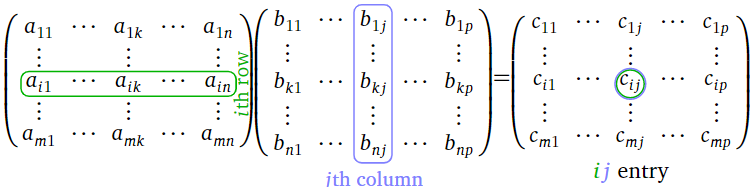
Figure \(\PageIndex{9}\)
The row-column rule for matrix-vector multiplication in Section 2.3, Recipe: The Row-Column Rule for Matrix-Vector Multiplication, says that if \(A\) has rows \(r_1,r_2,\ldots,r_m\) and \(x\) is a vector, then
\[Ax=\left(\begin{array}{c}—r_1— \\ —r_2— \\ \vdots \\ —r_m—\end{array}\right)x=\left(\begin{array}{c}r_1x \\ r_2x \\ \vdots \\ r_mx\end{array}\right).\nonumber\]
The Definition \(\PageIndex{3}\) of matrix multiplication is
\[A\left(\begin{array}{cccc}|&|&\quad&| \\ c_1&c_2&\cdots &c_p \\ |&|&\quad &| \end{array}\right)=\left(\begin{array}{cccc}|&|&\quad&| \\ Ac_1&Ac_2&\cdots &Ac_p \\ |&|&\quad &\end{array}\right).\nonumber\]
It follows that
\[\left(\begin{array}{c}—r_1— \\ —r_2— \\ \vdots \\ —r_m—\end{array}\right)\:\left(\begin{array}{cccc}|&|&\quad&| \\ c_1&c_2&\cdots &c_p \\ |&|&\quad &| \end{array}\right) =\left(\begin{array}{cccc}r_1c_1&r_1c_2&\cdots &r_1c_p \\ r_2c_1&r_2c_2&\cdots &r_2c_p \\ \vdots& \vdots &{}&\vdots \\ r_mc_1&r_mc_2 &\cdots &r_mc_p\end{array}\right).\nonumber\]
The row-column rule allows us to compute the product matrix one entry at a time:
\[\begin{aligned}\left(\begin{array}{ccc}\color{Green}{1}&\color{Green}{2}&\color{Green}{3} \\ \color{black}{4}&\color{black}{5}&\color{black}{6}\end{array}\right)\:\left(\begin{array}{cc}\color{blue}{1}&\color{black}{-3} \\ \color{blue}{2}&\color{black}{-2} \\ \color{blue}{3}&\color{black}{-1}\end{array}\right) &= \left(\begin{array}{cccccc} \color{Green}{1} \color{black}{\cdot}\color{blue}{1}&\color{black}{+}&\color{Green}{2}\color{black}{\cdot}\color{blue}{2}&\color{black}{+}&\color{Green}{3}\color{black}{\cdot}\color{blue}{3}&\fbox{ } \\ {}&{}&\fbox{ }&{}&{}&\fbox{ }\end{array}\right) = \left(\begin{array}{cc}\color{purple}{14}&\color{black}{\fbox{ }} \\ \fbox{ }&\fbox{ }\end{array}\right) \\ \left(\begin{array}{ccc}1&2&3 \\ \color{Green}{4}&\color{Green}{5}&\color{Green}{6}\end{array}\right)\left(\begin{array}{cc}\color{blue}{1}&\color{black}{-3}\\ \color{blue}{2}&\color{black}{-2} \\ \color{blue}{3}&\color{black}{-1}\end{array}\right)&=\left(\begin{array}{cccccc} {}&{}&\fbox{ }&{}&{}&\fbox{ } \\ \color{Green}{4}\color{black}{\cdot}\color{blue}{1}&\color{black}{+}&\color{Green}{5}\color{black}{\cdot}\color{blue}{2}&\color{black}{+}&\color{Green}{6}\color{black}{\cdot}\color{blue}{3}&\fbox{ }\end{array}\right)=\left(\begin{array}{cc}14&\fbox{ }\\ \color{purple}{32}&\color{black}{\fbox{ }}\end{array}\right) \end{aligned}\]
You should try to fill in the other two boxes!
Although matrix multiplication satisfies many of the properties one would expect (see the end of the section), one must be careful when doing matrix arithmetic, as there are several properties that are not satisfied in general.
- Matrix multiplication is not commutative: \(AB\) is not usually equal to \(BA\text{,}\) even when both products are defined and have the same size. See Example \(\PageIndex{9}\).
- Matrix multiplication does not satisfy the cancellation law: \(AB=AC\) does not imply \(B=C\text{,}\) even when \(A\neq 0\). For example,
\[\left(\begin{array}{cc}1&0\\0&0\end{array}\right)\left(\begin{array}{cc}1&2\\3&4\end{array}\right)=\left(\begin{array}{cc}1&2\\0&0\end{array}\right)=\left(\begin{array}{cc}1&0\\0&0\end{array}\right)\left(\begin{array}{cc}1&2\\5&6\end{array}\right).\nonumber\] - It is possible for \(AB=0\text{,}\) even when \(A\neq 0\) and \(B\neq 0\). For example,
\[\left(\begin{array}{cc}1&0\\1&0\end{array}\right)\left(\begin{array}{cc}0&0\\1&1\end{array}\right)=\left(\begin{array}{cc}0&0\\0&0\end{array}\right).\nonumber\]
While matrix multiplication is not commutative in general there are examples of matrices \(A\) and \(B\) with \(AB=BA\). For example, this always works when \(A\) is the zero matrix, or when \(A=B\). The reader is encouraged to find other examples.
Consider the matrices
\[A=\left(\begin{array}{cc}1&1\\0&1\end{array}\right)\quad\text{and}\quad B=\left(\begin{array}{cc}1&0\\1&1\end{array}\right),\nonumber\]
as in this Example \(\PageIndex{6}\). The matrix \(AB\) is
\[\left(\begin{array}{cc}1&1\\0&1\end{array}\right)\:\left(\begin{array}{cc}1&0\\1&1\end{array}\right)=\left(\begin{array}{cc}2&1\\1&1\end{array}\right),\nonumber\]
whereas the matrix \(BA\) is
\[\left(\begin{array}{cc}1&0\\1&1\end{array}\right)\:\left(\begin{array}{cc}1&1\\0&1\end{array}\right)=\left(\begin{array}{cc}1&1\\1&2\end{array}\right).\nonumber\]
In particular, we have
\[ AB \neq BA. \nonumber \]
And so matrix multiplication is not always commutative. It is not a coincidence that this example agrees with the previous Example \(\PageIndex{6}\); we are about to see that multiplication of matrices corresponds to composition of transformations.
Let \(T\colon\mathbb{R}^n \to\mathbb{R}^m \) and \(U\colon\mathbb{R}^p \to\mathbb{R}^n \) be linear transformations, and let \(A\) and \(B\) be their standard matrices, respectively. Recall that \(T\circ U(x)\) is the vector obtained by first applying \(U\) to \(x\text{,}\) and then \(T\).
On the matrix side, the standard matrix of \(T\circ U\) is the product \(AB\text{,}\) so \(T\circ U(x) = (AB)x\). By associativity of matrix multiplication, we have \((AB)x = A(Bx)\text{,}\) so the product \((AB)x\) can be computed by first multiplying \(x\) by \(B\text{,}\) then multipyling the product by \(A\).
Therefore, matrix multiplication happens in the same order as composition of transformations. In other words, both matrices and transformations are written in the order opposite from the order in which they act. But matrix multiplication and composition of transformations are written in the same order as each other: the matrix for \(T\circ U\) is \(AB\).
Composition and Matrix Multiplication
The point of this subsection is to show that matrix multiplication corresponds to composition of transformations, that is, the standard matrix for \(T \circ U\) is the product of the standard matrices for \(T\) and for \(U\). It should be hard to believe that our complicated formula for matrix multiplication actually means something intuitive such as “chaining two transformations together”!
Let \(T\colon\mathbb{R}^n \to\mathbb{R}^m \) and \(U\colon\mathbb{R}^p \to\mathbb{R}^n \) be linear transformations, and let \(A\) and \(B\) be their standard matrices, respectively, so \(A\) is an \(m\times n\) matrix and \(B\) is an \(n\times p\) matrix. Then \(T\circ U\colon\mathbb{R}^p \to\mathbb{R}^m \) is a linear transformation, and its standard matrix is the product \(AB\).
- Proof
-
First we verify that \(T\circ U\) is linear. Let \(u,v\) be vectors in \(\mathbb{R}^p \). Then
\[ \begin{aligned} T\circ U(u+v) &= T(U(u+v)) = T(U(u)+U(v)) \\ &= T(U(u))+T(U(v)) = T\circ U(u) + T\circ U(v). \end{aligned} \]
If \(c\) is a scalar, then
\[ T\circ U(cv) = T(U(cv)) = T(cU(v)) = cT(U(v)) = cT\circ U(v). \nonumber \]
Since \(T\circ U\) satisfies the two defining properties, Definition 3.3.1 in Section 3.3, it is a linear transformation.
Now that we know that \(T\circ U\) is linear, it makes sense to compute its standard matrix. Let \(C\) be the standard matrix of \(T\circ U\text{,}\) so \(T(x) = Ax,\) \(U(x) = Bx\text{,}\) and \(T\circ U(x) = Cx\). By Theorem 3.3.1 in Section 3.3, the first column of \(C\) is \(Ce_1\text{,}\) and the first column of \(B\) is \(Be_1\). We have
\[ T\circ U(e_1) = T(U(e_1)) = T(Be_1) = A(Be_1). \nonumber \]
By definition, the first column of the product \(AB\) is the product of \(A\) with the first column of \(B\text{,}\) which is \(Be_1\text{,}\) so
\[ Ce_1 = T\circ U(e_1) = A(Be_1) = (AB)e_1. \nonumber \]
It follows that \(C\) has the same first column as \(AB\). The same argument as applied to the \(i\)th standard coordinate vector \(e_i\) shows that \(C\) and \(AB\) have the same \(i\)th column; since they have the same columns, they are the same matrix.
The theorem justifies our choice of definition of the matrix product. This is the one and only reason that matrix products are defined in this way. To rephrase:
The matrix of the composition of two linear transformations is the product of the matrices of the transformations.
In Example 3.3.8 in Section 3.3, we showed that the standard matrix for the counterclockwise rotation of the plane by an angle of \(\theta\) is
\[A=\left(\begin{array}{cc}\cos\theta &-\sin\theta \\ \sin\theta &\cos\theta\end{array}\right).\nonumber\]
Let \(T\colon\mathbb{R}^2 \to\mathbb{R}^2 \) be counterclockwise rotation by \(45^\circ\text{,}\) and let \(U\colon\mathbb{R}^2 \to\mathbb{R}^2 \) be counterclockwise rotation by \(90^\circ\). The matrices \(A\) and \(B\) for \(T\) and \(U\) are, respectively,
\[\begin{aligned}A&=\left(\begin{array}{cc}\cos(45^\circ )&-\sin (45^\circ ) \\ \sin (45^\circ)&\cos (45^\circ)\end{array}\right) =\frac{1}{\sqrt{2}}\left(\begin{array}{cc}1&-1\\1&1\end{array}\right) \\ B&=\left(\begin{array}{cc}\cos(90^\circ )&-\sin (90^\circ ) \\ \sin (90^\circ)&\cos (90^\circ)\end{array}\right) =\left(\begin{array}{cc}0&-1\\1&0\end{array}\right). \end{aligned}\]
Here we used the trigonometric identities
\begin{align*} \cos(45^\circ) \amp= \frac 1{\sqrt2} \amp \sin(45^\circ) \amp= \frac 1{\sqrt2}\\ \cos(90^\circ) \amp= 0 \amp \sin(90^\circ) \amp= 1. \end{align*}
The standard matrix of the composition \(T\circ U\) is
\[AB=\frac{1}{\sqrt{2}}\left(\begin{array}{cc}1&-1\\1&1\end{array}\right)\left(\begin{array}{cc}0&-1\\1&0\end{array}\right)=\frac{1}{\sqrt{2}}\left(\begin{array}{cc}-1&-1\\1&-1\end{array}\right).\nonumber\]
This is consistent with the fact that \(T\circ U\) is counterclockwise rotation by \(90^\circ + 45^\circ = 135^\circ\text{:}\) we have
\[\left(\begin{array}{cc}\cos(135^\circ )&-\sin (135^\circ ) \\ \sin (135^\circ)&\cos (135^\circ)\end{array}\right) =\frac{1}{\sqrt{2}}\left(\begin{array}{cc}-1&-1\\1&-1\end{array}\right) \nonumber\]
because \(\cos(135^\circ) = -1/\sqrt2\) and \(\sin(135^\circ) = 1/\sqrt2\).
Derive the trigonometric identities
\[ \sin(\alpha\pm\beta) = \sin(\alpha)\cos(\beta) \pm \cos(\alpha)\sin(\beta) \nonumber \]
and
\[ \cos(\alpha\pm\beta) = \cos(\alpha)\cos(\beta) \mp \sin(\alpha)\sin(\beta) \nonumber \]
using the above Theorem \(\PageIndex{1}\) as applied to rotation transformations, as in the previous example.
Define \(T\colon\mathbb{R}^3 \to\mathbb{R}^2 \) and \(U\colon\mathbb{R}^2 \to\mathbb{R}^3 \) by
\[T(x)=\left(\begin{array}{ccc}1&1&0\\0&1&1\end{array}\right)x\quad\text{and}\quad U(x)=\left(\begin{array}{cc}1&0\\0&1\\1&0\end{array}\right)x.\nonumber\]
Their composition is a linear transformation \(T\circ U\colon\mathbb{R}^2 \to\mathbb{R}^2 \). By the Theorem \(\PageIndex{1}\), its standard matrix is
\[\left(\begin{array}{ccc}1&1&0\\0&1&1\end{array}\right)\left(\begin{array}{cc}1&0\\0&1\\1&0\end{array}\right)=\left(\begin{array}{cc}1&1\\1&1\end{array}\right),\nonumber\]
as we computed in the above Example \(\PageIndex{7}\).
Let \(S\colon\mathbb{R}^3 \to\mathbb{R}^3 \) be the linear transformation that first reflects over the \(xy\)-plane and then projects onto the \(yz\)-plane, as in Example 3.3.10 in Section 3.3. The transformation \(S\) is the composition \(T\circ U\text{,}\) where \(U\colon\mathbb{R}^3 \to\mathbb{R}^3 \) is the transformation that reflects over the \(xy\)-plane, and \(T\colon\mathbb{R}^3 \to\mathbb{R}^3 \) is the transformation that projects onto the \(yz\)-plane.
Let us compute the matrix \(B\) for \(U\).
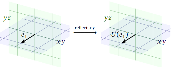
Figure \(\PageIndex{11}\)
Since \(e_1\) lies on the \(xy\)-plane, reflecting it over the \(xy\)-plane does not move it:
\[ U(e_1) = \left(\begin{array}{c}1\\0\\0\end{array}\right). \nonumber \]
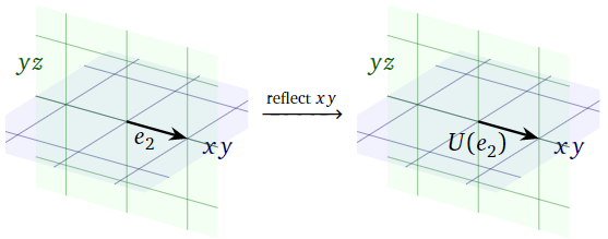
Figure \(\PageIndex{12}\)
Since \(e_2\) lies on the \(xy\)-plane, reflecting over the \(xy\)-plane does not move it either:
\[ U(e_2) = e_2 = \left(\begin{array}{c}0\\1\\0\end{array}\right). \nonumber \]
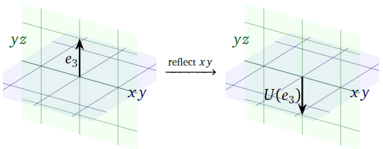
Figure \(\PageIndex{13}\)
Since \(e_3\) is perpendicular to the \(xy\)-plane, reflecting over the \(xy\)-plane takes \(e_3\) to its negative:
\[ U(e_3) = -e_3 = \left(\begin{array}{c}0\\0\\-1\end{array}\right). \nonumber \]
We have computed all of the columns of \(B\text{:}\)
\[B=\left(\begin{array}{ccc}|&|&| \\ U(e_1)&U(e_2)&U(e_3) \\ |&|&|\end{array}\right)=\left(\begin{array}{ccc}1&0&0\\0&1&0\\0&0&-1\end{array}\right).\nonumber\]
By a similar method, we find
\[A=\left(\begin{array}{ccc}0&0&0\\0&1&0\\0&0&1\end{array}\right).\nonumber\]
It follows that the matrix for \(S = T\circ U\) is
\[\begin{aligned} AB&=\left(\begin{array}{ccc}0&0&0\\0&1&0\\0&0&1\end{array}\right)\:\left(\begin{array}{ccc}1&0&0\\0&1&0\\0&0&-1\end{array}\right) \\ &=\left(\left(\begin{array}{ccc}0&0&0\\0&1&0\\0&0&1\end{array}\right)\left(\begin{array}{c}1\\0\\0\end{array}\right)\:\:\left(\begin{array}{ccc}0&0&0\\0&1&0\\0&0&1\end{array}\right)\left(\begin{array}{c}0\\1\\0\end{array}\right)\:\:\left(\begin{array}{ccc}0&0&0\\0&1&0\\0&0&1\end{array}\right)\left(\begin{array}{c}0\\0\\-1\end{array}\right)\right) \\ &=\left(\begin{array}{ccc}0&0&0\\0&1&0\\0&0&-1\end{array}\right),\end{aligned}\]
as we computed in Example 3.3.10 in Section 3.3.
Recall from Definition 3.3.2 in Section 3.3 that the identity matrix is the \(n\times n\) matrix \(I_n\) whose columns are the standard coordinate vectors in \(\mathbb{R}^n \). The identity matrix is the standard matrix of the identity transformation: that is, \(x = \operatorname{Id}_{\mathbb{R}^n }(x) = I_nx\) for all vectors \(x\) in \(\mathbb{R}^n \). For any linear transformation \(T : \mathbb{R}^n \to \mathbb{R}^m \) we have
\[ I_{\mathbb{R}^m } \circ T = T \nonumber \]
and by the same token we have for any \(m \times n\) matrix \(A\) we have
\[ I_mA=A\text{.} \nonumber \]
Similarly, we have \(T \circ I_{\mathbb{R}^n } = T\) and \(AI_n=A\).
The algebra of transformations and matrices
In this subsection we describe two more operations that one can perform on transformations: addition and scalar multiplication. We then translate these operations into the language of matrices. This is analogous to what we did for the composition of linear transformations, but much less subtle.
- Let \(T,U\colon\mathbb{R}^n \to\mathbb{R}^m \) be two transformations. Their sum is the transformation \(T+U\colon\mathbb{R}^n \to\mathbb{R}^m \) defined by
\[(T+U)(x)=T(x)+U(x).\nonumber\]
Note that addition of transformations is only defined when both transformations have the same domain and codomain. - Let \(T\colon\mathbb{R}^n \to\mathbb{R}^m \) be a transformation, and let \(c\) be a scalar. The scalar product of \(c\) with \(T\) is the transformation \(cT\colon\mathbb{R}^n \to\mathbb{R}^m \) defined by
\[(cT)(x)=c\cdot T(x).\nonumber\]
To emphasize, the sum of two transformations \(T,U\colon\mathbb{R}^n \to\mathbb{R}^m \) is another transformation called \(T+U\text{;}\) its value on an input vector \(x\) is the sum of the outputs of \(T\) and \(U\). Similarly, the product of \(T\) with a scalar \(c\) is another transformation called \(cT\text{;}\) its value on an input vector \(x\) is the vector \(c\cdot T(x)\).
Define \(f\colon \mathbb{R} \to\mathbb{R} \) by \(f(x) = x^2\) and \(g\colon \mathbb{R} \to\mathbb{R} \) by \(g(x) = x^3\). The sum \(f+g\colon \mathbb{R} \to\mathbb{R} \) is the transformation defined by the rule
\[ (f+g)(x) = f(x) + g(x) = x^2 + x^3. \nonumber \]
For instance, \((f+g)(-2) = (-2)^2 + (-2)^3 = -4\).
Define \(\exp\colon \mathbb{R} \to\mathbb{R} \) by \(\exp(x) = e^x\). The product \(2\exp\colon \mathbb{R} \to\mathbb{R} \) is the transformation defined by the rule
\[ (2\exp)(x) = 2\cdot\exp(x) = 2e^x. \nonumber \]
For instance, \((2\exp)(1) = 2\cdot\exp(1) = 2e\).
Let \(S,T,U\colon\mathbb{R}^n \to\mathbb{R}^m \) be transformations and let \(c,d\) be scalars. The following properties are easily verified:
\begin{align*} T + U \amp= U + T \amp S + (T + U) \amp= (S + T) + U\\ c(T + U) \amp= cT + cU \amp (c + d)T \amp= cT + dT\\ c(dT) \amp= (cd)T \amp T + 0 \amp= T \end{align*}
In one of the above properties, we used \(0\) to denote the transformation \(\mathbb{R}^n \to\mathbb{R}^m \) that is zero on every input vector: \(0(x) = 0\) for all \(x\). This is called the zero transformation.
We now give the analogous operations for matrices.
- The sum of two \(m\times n\) matrices is the matrix obtained by summing the entries of \(A\) and \(B\) individually:
\[\left(\begin{array}{ccc}a_{11}&a_{12}&a_{13} \\ a_{21}&a_{22}&a_{23}\end{array}\right)+\left(\begin{array}{ccc}b_{11}&b_{12}&b_{13}\\b_{21}&b_{22}&b_{23}\end{array}\right)=\left(\begin{array}{ccc}a_{11}+b_{11}&a_{12}+b_{12}&a_{13}+b_{13} \\ a_{21}+b_{21}&a_{22}+b_{22}&a_{23}+b_{23}\end{array}\right)\nonumber\]
In other words, the \(i,j\) entry of \(A+B\) is the sum of the \(i,j\) entries of \(A\) and \(B\). Note that addition of matrices is only defined when both matrices have the same size. - The scalar product of a scalar \(c\) with a matrix \(A\) is obtained by scaling all entries of \(A\) by \(c\text{:}\)
\[\color{red}{c}\color{black}{\left(\begin{array}{ccc}a_{11}&a_{12}&a_{13}\\a_{21}&a_{22}&a_{23}\end{array}\right)=}\left(\begin{array}{ccc}\color{red}{c}\color{black}{a_{11}}&\color{red}{a}\color{black}{a_{12}}&\color{red}{c}\color{black}{a_{13}} \\ \color{red}{c}\color{black}{a_{21}}&\color{red}{c}\color{black}{a_{22}}&\color{red}{c}\color{black}{a_{23}}\end{array}\right)\nonumber\]
In other words, the \(i,j\) entry of \(cA\) is \(c\) times the \(i,j\) entry of \(A\).
Let \(T,U\colon\mathbb{R}^n \to\mathbb{R}^m \) be linear transformations with standard matrices \(A,B\text{,}\) respectively, and let \(c\) be a scalar.
- The standard matrix for \(T+U\) is \(A+B\).
- The standard matrix for \(cT\) is \(cA\).
In view of the above fact, the following properties, Note \(\PageIndex{7}\), are consequences of the corresponding properties 29 of transformations. They are easily verified directly from the definitions as well.
Let \(A,B,C\) be \(m\times n\) matrices and let \(c,d\) be scalars. Then:
\begin{align*} A + B \amp= B + A \amp C + (A + B) \amp= (C + A) + B\\ c(A + B) \amp= cA + cB \amp (c + d)A \amp= cA + dA\\ c(dA) \amp= (cd)A \amp A + 0 \amp= A \end{align*}
In one of the above properties, we used \(0\) to denote the \(m\times n\) matrix whose entries are all zero. This is the standard matrix of the zero transformation, and is called the zero matrix.
We can also combine addition and scalar multiplication of matrices with multiplication of matrices. Since matrix multiplication corresponds to composition of transformations (Theorem \(\PageIndex{1}\)), the following properties are consequences of the corresponding properties, Note \(\PageIndex{2}\) of transformations.
Let \(A,B,C\) be matrices and let \(c\) be a scalar. Suppose that \(A\) is an \(m\times n\) matrix, and that in each of the following identities, the sizes of \(B\) and \(C\) are compatible when necessary for the product to be defined. Then:
\begin{align*} C(A+B) \amp= C A+C B \amp (A + B) C \amp= A C + B C \amp\\ c(A B) \amp= (cA) B \amp c(A B) \amp= A(cB)\\ A I_n \amp= A \amp I_m A \amp= A\\ (A B)C \amp= A (BC) \amp \end{align*}
Most of the above properties are easily verified directly from the definitions. The associativity property \((AB)C=A(BC)\text{,}\) however, is not (try it!). It is much easier to prove by relating matrix multiplication to composition of transformations, and using the obvious fact that composition of transformations is associative.