2.3: Equations, Matricies and Transformations

Up to now we have used matrices to solve systems of linear equations by manipulating the rows of the augmented matrix. In this section we introduce a different way of describing linear systems that makes more use of the coefficient matrix of the system and leads to a useful way of “multiplying” matrices.

Vectors

It is a well-known fact in analytic geometry that two points in the plane with coordinates \((a_{1}, a_{2})\) and \((b_{1}, b_{2})\) are equal if and only if \(a_{1} = b_{1}\) and \(a_{2} = b_{2}\). Moreover, a similar condition applies to points \((a_{1}, a_{2}, a_{3})\) in space. We extend this idea as follows.

An ordered sequence \((a_{1}, a_{2}, \dots, a_{n})\) of real numbers is called an ordered \(\boldsymbol{n}\)-tuple. The word “ordered” here reflects our insistence that two ordered \(n\)-tuples are equal if and only if corresponding entries are the same. In other words,

\[(a_{1}, a_{2}, \dots, a_{n}) = (b_{1}, b_{2}, \dots, b_{n}) \quad \mbox{if and only if} \quad a_{1} = b_{1}, a_{2} = b_{2}, \dots, \mbox{ and } a_{n} = b_{n}. \nonumber \]

Thus the ordered \(2\)-tuples and \(3\)-tuples are just the ordered pairs and triples familiar from geometry.

Definition: \(\PageIndex{1}\)

The set \(\mathbb{R}^n\) of ordered \(n\)-tuples of real numbers002606 Let \(\mathbb{R}\) denote the set of all real numbers. The set of all ordered \(n\)-tuples from \(\mathbb{R}\) has a special notation:

\[\mathbb{R}^{n} \mbox{ denotes the set of all ordered }n\mbox{-tuples of real numbers.} \nonumber \]

There are two commonly used ways to denote the \(n\)-tuples in \(\mathbb{R}^{n}\): As rows \((r_{1}, r_{2}, \dots, r_{n})\) or columns \(\left[ \begin{array}{c} r_{1} \\ r_{2} \\ \vdots \\ r_{n} \end{array} \right]\); the notation we use depends on the context. In any event they are called vectors or \(n\)-vectors and will be denoted using bold type such as \(\mathbf{x}\) or \(\mathbf{v}\). For example, an \(m \times n\) matrix \(A\) will be written as a row of columns:

\[A = \left[ \begin{array}{cccc} \mathbf{a}_{1} & \mathbf{a}_{2} & \cdots & \mathbf{a}_{n} \end{array} \right] \mbox{ where } \mathbf{a}_{j} \mbox{ denotes column } j \mbox{ of } A \mbox{ for each } j. \nonumber \]

If \(\mathbf{x}\) and \(\mathbf{y}\) are two \(n\)-vectors in \(\mathbb{R}^n\), it is clear that their matrix sum \(\mathbf{x} + \mathbf{y}\) is also in \(\mathbb{R}^n\) as is the scalar multiple \(k\mathbf{x}\) for any real number \(k\). We express this observation by saying that \(\mathbb{R}^n\) is closed under addition and scalar multiplication. In particular, all the basic properties in Theorem [thm:002170] are true of these \(n\)-vectors. These properties are fundamental and will be used frequently below without comment. As for matrices in general, the \(n \times 1\) zero matrix is called the zero \(\boldsymbol{n}\)-vector in \(\mathbb{R}^n\) and, if \(\mathbf{x}\) is an \(n\)-vector, the \(n\)-vector \(-\mathbf{x}\) is called the negative \(\mathbf{x}\).

Of course, we have already encountered these \(n\)-vectors in Section [sec:1_3] as the solutions to systems of linear equations with \(n\) variables. In particular we defined the notion of a linear combination of vectors and showed that a linear combination of solutions to a homogeneous system is again a solution. Clearly, a linear combination of \(n\)-vectors in \(\mathbb{R}^n\) is again in \(\mathbb{R}^n\), a fact that we will be using.

Matrix-Vector Multiplication

Given a system of linear equations, the left sides of the equations depend only on the coefficient matrix \(A\) and the column \(\mathbf{x}\) of variables, and not on the constants. This observation leads to a fundamental idea in linear algebra: We view the left sides of the equations as the “product” \(A\mathbf{x}\) of the matrix \(A\) and the vector \(\mathbf{x}\). This simple change of perspective leads to a completely new way of viewing linear systems—one that is very useful and will occupy our attention throughout this book.

To motivate the definition of the “product” \(A\mathbf{x}\), consider first the following system of two equations in three variables:

\[\label{eq:linsystem} \begin{array}{rrrrrrr} ax_{1} & + & bx_{2} & + & cx_{3} & = & b_{1} \\ a^{\prime}x_{1} & + & b^{\prime}x_{2} & + & c^{\prime}x_{3} & = & b_{1} \end{array} \]

and let \(A = \left[ \begin{array}{ccc} a & b & c \\ a^\prime & b^\prime & c^\prime \end{array} \right]\), \(\mathbf{x} = \left[ \begin{array}{c} x_{1} \\ x_{2} \\ x_{3} \end{array} \right]\), \(\mathbf{b} = \left[ \begin{array}{c} b_{1} \\ b_{2} \end{array} \right]\) denote the coefficient matrix, the variable matrix, and the constant matrix, respectively. The system ([eq:linsystem]) can be expressed as a single vector equation

\[\left[ \begin{array}{rrrrr} ax_{1} & + & bx_{2} & + & cx_{3} \\ a^\prime x_{1} & + & b^\prime x_{2} & + & c^\prime x_{3} \end{array} \right] = \left[ \begin{array}{c} b_{1} \\ b_{2} \end{array} \right] \nonumber \]

which in turn can be written as follows:

\[x_{1} \left[ \begin{array}{c} a \\ a^\prime \end{array} \right] + x_{2} \left[ \begin{array}{c} b \\ b^\prime \end{array} \right] + x_{3} \left[ \begin{array}{c} c \\ c^\prime \end{array} \right] = \left[ \begin{array}{c} b_{1} \\ b_{2} \end{array} \right] \nonumber \]

Now observe that the vectors appearing on the left side are just the columns

\[\mathbf{a}_{1} = \left[ \begin{array}{c} a \\ a^\prime \end{array} \right], \mathbf{a}_{2} = \left[ \begin{array}{c} b \\ b^\prime \end{array} \right], \mbox{ and } \mathbf{a}_{3} = \left[ \begin{array}{c} c \\ c^\prime \end{array} \right] \nonumber \]

of the coefficient matrix \(A\). Hence the system ([eq:linsystem]) takes the form

\[\label{eq:linsystem2} x_{1}\mathbf{a}_{1} + x_{2}\mathbf{a}_{2} + x_{3}\mathbf{a}_{3} = \mathbf{b} \]

This shows that the system ([eq:linsystem]) has a solution if and only if the constant matrix \(\mathbf{b}\) is a linear combination¹ of the columns of \(A\), and that in this case the entries of the solution are the coefficients \(x_{1}\), \(x_{2}\), and \(x_{3}\) in this linear combination.

Moreover, this holds in general. If \(A\) is any \(m \times n\) matrix, it is often convenient to view \(A\) as a row of columns. That is, if \(\mathbf{a}_{1}, \mathbf{a}_{2}, \dots, \mathbf{a}_{n}\) are the columns of \(A\), we write

\[A = \left[ \begin{array}{cccc} \mathbf{a}_{1} & \mathbf{a}_{2} & \cdots & \mathbf{a}_{n} \end{array} \right] \nonumber \]

and say that \(A = \left[ \begin{array}{cccc} \mathbf{a}_{1} & \mathbf{a}_{2} & \cdots & \mathbf{a}_{n} \end{array} \right]\) is given in terms of its columns.

Now consider any system of linear equations with \(m \times n\) coefficient matrix \(A\). If \(\mathbf{b}\) is the constant matrix of the system, and if \(\mathbf{x} = \left[ \begin{array}{c} x_{1} \\ x_{2} \\ \vdots \\ x_{n} \end{array} \right]\) is the matrix of variables then, exactly as above, the system can be written as a single vector equation

\[\label{eq:singlevector} x_{1}\mathbf{a}_{1} + x_{2}\mathbf{a}_{2} + \dots + x_{n}\mathbf{a}_{n} = \mathbf{b} \]

Example \(\PageIndex{1}\)

Write the system \(\left\lbrace \begin{array}{rrrrrrr} 3x_{1} & + & 2x_{2} & - & 4x_{3} & = & 0 \\ x_{1} & - & 3x_{2} & + & x_{3} & = & 3 \\ & & x_{2} & - & 5x_{3} & = & -1 \end{array} \right.\) in the form given in (Eq. \(\PageIndex{4}\)).

Solution

\[x_{1} \left[ \begin{array}{r} 3 \\ 1 \\ 0 \end{array} \right] + x_{2} \left[ \begin{array}{r} 2 \\ -3 \\ 1 \end{array} \right] + x_{3} \left[ \begin{array}{r} -4 \\ 1 \\ -5 \end{array} \right] = \left[ \begin{array}{r} 0 \\ 3 \\ -1 \end{array} \right] \nonumber \]

As mentioned above, we view the left side of Equation \(\PageIndex{4}\) as the product of the matrix \(A\) and the vector \(\mathbf{x}\). This basic idea is formalized in the following definition:

Definition: Matrix-Vector Multiplication \(\PageIndex{2}\)

Let \(A = \left[ \begin{array}{cccc} \mathbf{a}_{1} & \mathbf{a}_{2} & \cdots & \mathbf{a}_{n} \end{array} \right]\) be an \(m \times n\) matrix, written in terms of its columns \(\mathbf{a}_{1}, \mathbf{a}_{2}, \dots, \mathbf{a}_{n}\). If \(\mathbf{x} = \left[ \begin{array}{c} x_{1} \\ x_{2} \\ \vdots \\ x_{n} \end{array} \right]\) is any n-vector, the product \(A\mathbf{x}\) is defined to be the \(m\)-vector given by:

\[A\mathbf{x} = x_{1}\mathbf{a}_{1} + x_{2}\mathbf{a}_{2} + \cdots + x_{n}\mathbf{a}_{n} \nonumber \]

In other words, if \(A\) is \(m \times n\) and \(\mathbf{x}\) is an \(n\)-vector, the product \(A\mathbf{x}\) is the linear combination of the columns of \(A\) where the coefficients are the entries of \(\mathbf{x}\) (in order).

Note that if \(A\) is an \(m \times n\) matrix, the product \(A\mathbf{x}\) is only defined if \(\mathbf{x}\) is an \(n\)-vector and then the vector \(A\mathbf{x}\) is an \(m\)-vector because this is true of each column \(\mathbf{a}_{j}\) of \(A\). But in this case the system of linear equations with coefficient matrix \(A\) and constant vector \(\mathbf{b}\) takes the form of a single matrix equation

\[A\mathbf{x} = \mathbf{b} \nonumber \]

The following theorem combines Definition \(\PageIndex{2}\) and equation Eq. \(\PageIndex{4}\)and summarizes the above discussion. Recall that a system of linear equations is said to be consistent if it has at least one solution.

Theorem \(\PageIndex{1}\)

1. Every system of linear equations has the form \(A\mathbf{x} = \mathbf{b}\) where \(A\) is the coefficient matrix, \(\mathbf{b}\) is the constant matrix, and \(\mathbf{x}\) is the matrix of variables.
2. The system \(A\mathbf{x} = \mathbf{b}\) is consistent if and only if \(\mathbf{b}\) is a linear combination of the columns of \(A\).
3. \[x_{1}\mathbf{a}_{1} + x_{2}\mathbf{a}_{2} + \cdots + x_{n}\mathbf{a}_{n} = \mathbf{b} \nonumber \]

A system of linear equations in the form \(A\mathbf{x} = \mathbf{b}\) as in (1) of Theorem \(\PageIndex{1}\) is said to be written in matrix form. This is a useful way to view linear systems as we shall see.

Theorem \(\PageIndex{1}\) transforms the problem of solving the linear system \(A\mathbf{x} = \mathbf{b}\) into the problem of expressing the constant matrix \(B\) as a linear combination of the columns of the coefficient matrix \(A\). Such a change in perspective is very useful because one approach or the other may be better in a particular situation; the importance of the theorem is that there is a choice.

Example \(\PageIndex{2}\)

If \(A = \left[ \begin{array}{rrrr} 2 & -1 & 3 & 5 \\ 0 & 2 & -3 & 1 \\ -3 & 4 & 1 & 2 \end{array} \right]\) and \(\mathbf{x} = \left[ \begin{array}{r} 2 \\ 1 \\ 0 \\ -2 \end{array} \right]\), compute \(A\mathbf{x}\).

Solution

By Definition [def:002668]: \(A\mathbf{x} = 2 \left[ \begin{array}{r} 2 \\ 0 \\ -3 \end{array} \right] + 1 \left[ \begin{array}{r} -1 \\ 2 \\ 4 \end{array} \right] + 0 \left[ \begin{array}{r} 3 \\ -3 \\ 1 \end{array} \right] - 2 \left[ \begin{array}{r} 5 \\ 1 \\ 2 \end{array} \right] = \left[ \begin{array}{r} -7 \\ 0 \\ -6 \end{array} \right]\).

Example \(\PageIndex{3}\)

Given columns \(\mathbf{a}_{1}\), \(\mathbf{a}_{2}\), \(\mathbf{a}_{3}\), and \(\mathbf{a}_{4}\) in \(\mathbb{R}^3\), write \(2\mathbf{a}_{1} - 3\mathbf{a}_{2} + 5\mathbf{a}_{3} + \mathbf{a}_{4}\) in the form \(A\mathbf{x}\) where \(A\) is a matrix and \(\mathbf{x}\) is a vector.

Solutio

Here the column of coefficients is \(\mathbf{x} = \left[ \begin{array}{r} 2 \\ -3 \\ 5 \\ 1 \end{array} \right].\) Hence Definition [def:002668] gives

\[A\mathbf{x} = 2\mathbf{a}_{1} - 3\mathbf{a}_{2} + 5\mathbf{a}_{3} + \mathbf{a}_{4} \nonumber \]

where \(A = \left[ \begin{array}{cccc} \mathbf{a}_{1} & \mathbf{a}_{2} & \mathbf{a}_{3} & \mathbf{a}_{4} \end{array} \right]\) is the matrix with \(\mathbf{a}_{1}\), \(\mathbf{a}_{2}\), \(\mathbf{a}_{3}\), and \(\mathbf{a}_{4}\) as its columns.

Example \(\PageIndex{4}\)

Let \(A = \left[ \begin{array}{cccc} \mathbf{a}_{1} & \mathbf{a}_{2} & \mathbf{a}_{3} & \mathbf{a}_{4} \end{array} \right]\) be the \(3 \times 4\) matrix given in terms of its columns \(\mathbf{a}_{1} = \left[ \begin{array}{r} 2 \\ 0 \\ -1 \end{array} \right]\), \(\mathbf{a}_{2} = \left[ \begin{array}{r} 1 \\ 1 \\ 1 \end{array} \right]\), \(\mathbf{a}_{3} = \left[ \begin{array}{r} 3 \\ -1 \\ -3 \end{array} \right]\), and \(\mathbf{a}_{4} = \left[ \begin{array}{r} 3 \\ 1 \\ 0 \end{array} \right]\). In each case below, either express \(\mathbf{b}\) as a linear combination of \(\mathbf{a}_{1}\), \(\mathbf{a}_{2}\), \(\mathbf{a}_{3}\), and \(\mathbf{a}_{4}\), or show that it is not such a linear combination. Explain what your answer means for the corresponding system \(A\mathbf{x} = \mathbf{b}\) of linear equations.

1. \(\mathbf{b} = \left[ \begin{array}{r} 1 \\ 2 \\ 3 \end{array} \right]\)
2. \(\mathbf{b} = \left[ \begin{array}{r} 4 \\ 2 \\ 1 \end{array} \right]\)

Solution

By Theorem [thm:002684], \(\mathbf{b}\) is a linear combination of \(\mathbf{a}_{1}\), \(\mathbf{a}_{2}\), \(\mathbf{a}_{3}\), and \(\mathbf{a}_{4}\) if and only if the system \(A\mathbf{x} = \mathbf{b}\) is consistent (that is, it has a solution). So in each case we carry the augmented matrix \(\left[ A|\mathbf{b} \right]\) of the system \(A\mathbf{x} = \mathbf{b}\) to reduced form.

1. Here \(\left[ \begin{array}{rrrr|r} 2 & 1 & 3 & 3 & 1 \\ 0 & 1 & -1 & 1 & 2 \\ -1 & 1 & -3 & 0 & 3 \end{array} \right] \rightarrow \left[ \begin{array}{rrrr|r} 1 & 0 & 2 & 1 & 0 \\ 0 & 1 & -1 & 1 & 0 \\ 0 & 0 & 0 & 0 & 1 \end{array} \right]\), so the system \(A\mathbf{x} = \mathbf{b}\) has no solution in this case. Hence \(\mathbf{b}\) is not a linear combination of \(\mathbf{a}_{1}\), \(\mathbf{a}_{2}\), \(\mathbf{a}_{3}\), and \(\mathbf{a}_{4}\).
2. Now \(\left[ \begin{array}{rrrr|r} 2 & 1 & 3 & 3 & 4 \\ 0 & 1 & -1 & 1 & 2 \\ -1 & 1 & -3 & 0 & 1 \end{array} \right] \rightarrow \left[ \begin{array}{rrrr|r} 1 & 0 & 2 & 1 & 1 \\ 0 & 1 & -1 & 1 & 2 \\ 0 & 0 & 0 & 0 & 0 \end{array} \right]\), so the system \(A\mathbf{x} = \mathbf{b}\) is consistent.

Thus \(\mathbf{b}\) is a linear combination of \(\mathbf{a}_{1}\), \(\mathbf{a}_{2}\), \(\mathbf{a}_{3}\), and \(\mathbf{a}_{4}\) in this case. In fact the general solution is \(x_{1} = 1 - 2s - t\), \(x_{2} = 2 + s - t\), \(x_{3} = s\), and \(x_{4} = t\) where \(s\) and \(t\) are arbitrary parameters. Hence \(x_{1}\mathbf{a}_{1} + x_{2}\mathbf{a}_{2} + x_{3}\mathbf{a}_{3} + x_{4}\mathbf{a}_{4} = \mathbf{b} = \left[ \begin{array}{r} 4 \\ 2 \\ 1 \end{array} \right]\) for any choice of \(s\) and \(t\). If we take \(s = 0\) and \(t = 0\), this becomes \(\mathbf{a}_{1} + 2\mathbf{a}_{2} = \mathbf{b}\), whereas taking \(s = 1 = t\) gives \(-2\mathbf{a}_{1} + 2\mathbf{a}_{2} + \mathbf{a}_{3} + \mathbf{a}_{4} = \mathbf{b}\).

Example \(\PageIndex{5}\)

Taking \(A\) to be the zero matrix, we have \(0\mathbf{x} = \mathbf{0}\) for all vectors \(\mathbf{x}\) by Definition [def:002668] because every column of the zero matrix is zero. Similarly, \(A\mathbf{0} = \mathbf{0}\) for all matrices \(A\) because every entry of the zero vector is zero.

Example \(\PageIndex{6}\)

If \(I = \left[ \begin{array}{rrr} 1 & 0 & 0 \\ 0 & 1 & 0 \\ 0 & 0 & 1 \end{array} \right]\), show that \(I\mathbf{x} = \mathbf{x}\) for any vector \(\mathbf{x}\) in \(\mathbb{R}^3\).

Solution

If \(\mathbf{x} = \left[ \begin{array}{r} x_{1} \\ x_{2} \\ x_{3} \end{array} \right]\) then Definition [\(\PageIndex{2}\) gives

\[I\mathbf{x} = x_{1} \left[ \begin{array}{r} 1 \\ 0 \\ 0 \\ \end{array} \right] + x_{2} \left[ \begin{array}{r} 0 \\ 1 \\ 0 \\ \end{array} \right] + x_{3} \left[ \begin{array}{r} 0 \\ 0 \\ 1 \\ \end{array} \right] = \left[ \begin{array}{r} x_{1} \\ 0 \\ 0 \\ \end{array} \right] + \left[ \begin{array}{r} 0 \\ x_{2} \\ 0 \\ \end{array} \right] + \left[ \begin{array}{r} 0 \\ 0 \\ x_{3} \\ \end{array} \right] = \left[ \begin{array}{r} x_{1} \\ x_{2} \\ x_{3} \\ \end{array} \right] = \mathbf{x} \nonumber \]

The matrix \(I\) in Example\(\PageIndex{6}\) is called the \(3 \times 3\) identity matrix, and we will encounter such matrices again in Example [exa:002949] below. Before proceeding, we develop some algebraic properties of matrix-vector multiplication that are used extensively throughout linear algebra.

Theorem \(\PageIndex{2}\)

Let \(A\) and \(B\) be \(m \times n\) matrices, and let \(\mathbf{x}\) and \(\mathbf{y}\) be \(n\)-vectors in \(\mathbb{R}^n\). Then:

1. \(A(\mathbf{x} + \mathbf{y}) = A\mathbf{x} + A\mathbf{y}\).
2. \(A(a\mathbf{x}) = a(A\mathbf{x}) = (aA)\mathbf{x}\) for all scalars \(a\).
3. \((A + B)\mathbf{x} = A\mathbf{x} + B\mathbf{x}\).

Proof. We prove (3); the other verifications are similar and are left as exercises. Let \(A = \left[ \begin{array}{cccc} \mathbf{a}_{1} & \mathbf{a}_{2} & \cdots & \mathbf{a}_{n} \end{array} \right]\) and \(B = \left[ \begin{array}{cccc} \mathbf{b}_{1} & \mathbf{b}_{2} & \cdots & \mathbf{b}_{n} \end{array} \right]\) be given in terms of their columns. Since adding two matrices is the same as adding their columns, we have

\[A + B = \left[ \begin{array}{cccc} \mathbf{a}_{1} + \mathbf{b}_{1} & \mathbf{a}_{2} + \mathbf{b}_{2} & \cdots & \mathbf{a}_{n} + \mathbf{b}_{n} \end{array} \right] \nonumber \]

If we write \(\mathbf{x} = \left[ \begin{array}{c} x_{1} \\ x_{2} \\ \vdots \\ x_{n} \end{array} \right]\) Definition [def:002668] gives

\[\begin{aligned} (A + B)\mathbf{x} &= x_{1}(\mathbf{a}_{1} + \mathbf{b}_{1}) + x_{2}(\mathbf{a}_{2} + \mathbf{b}_{2}) + \dots + x_{n}(\mathbf{a}_{n} + \mathbf{b}_{n}) \\ &= (x_{1}\mathbf{a}_{1} + x_{2}\mathbf{a}_{2} + \dots + x_{n}\mathbf{a}_{n}) + (x_{1}\mathbf{b}_{1} + x_{2}\mathbf{b}_{2} + \dots + x_{n}\mathbf{b}_{n})\\ &= A\mathbf{x} + B\mathbf{x}\end{aligned} \nonumber \]

Theorem (\PageIndex{2}\) allows matrix-vector computations to be carried out much as in ordinary arithmetic. For example, for any \(m \times n\) matrices \(A\) and \(B\) and any \(n\)-vectors \(\mathbf{x}\) and \(\mathbf{y}\), we have:

\[A(2\mathbf{x} - 5\mathbf{y}) = 2A\mathbf{x} - 5A\mathbf{y} \quad \mbox{ and } \quad (3A -7B)\mathbf{x} = 3A\mathbf{x} - 7B\mathbf{x} \nonumber \]

We will use such manipulations throughout the book, often without mention.

Linear Equations

Theorem [thm:002811] also gives a useful way to describe the solutions to a system

\[A\mathbf{x} = \mathbf{b} \nonumber \]

of linear equations. There is a related system

\[A\mathbf{x} = \mathbf{0} \nonumber \]

called the associated homogeneous system, obtained from the original system \(A\mathbf{x} = \mathbf{b}\) by replacing all the constants by zeros. Suppose \(\mathbf{x}_{1}\) is a solution to \(A\mathbf{x} = \mathbf{b}\) and \(\mathbf{x}_{0}\) is a solution to \(A\mathbf{x} = \mathbf{0}\) (that is \(A\mathbf{x}_{1} = \mathbf{b}\) and \(A\mathbf{x}_{0} = \mathbf{0}\)). Then \(\mathbf{x}_{1} + \mathbf{x}_{0}\) is another solution to \(A\mathbf{x} = \mathbf{b}\). Indeed, Theorem [thm:002811] gives

\[A(\mathbf{x}_{1} + \mathbf{x}_{0}) = A\mathbf{x}_{1} + A\mathbf{x}_{0} = \mathbf{b} + \mathbf{0} = \mathbf{b} \nonumber \]

This observation has a useful converse.

Theorem \(\PageIndex{3}\)

Suppose \(\mathbf{x}_{1}\) is any particular solution to the system \(A\mathbf{x} = \mathbf{b}\) of linear equations. Then every solution \(\mathbf{x}_{2}\) to \(A\mathbf{x} = \mathbf{b}\) has the form

\[\mathbf{x}_{2} = \mathbf{x}_{0} + \mathbf{x}_{1} \nonumber \]

for some solution \(\mathbf{x}_{0}\) of the associated homogeneous system \(A\mathbf{x} = \mathbf{0}\).

Proof. Suppose \(\mathbf{x}_{2}\) is also a solution to \(A\mathbf{x} = \mathbf{b}\), so that \(A\mathbf{x}_{2} = \mathbf{b}\). Write \(\mathbf{x}_{0} = \mathbf{x}_{2} - \mathbf{x}_{1}\). Then \(\mathbf{x}_{2} = \mathbf{x}_{0} + \mathbf{x}_{1}\) and, using Theorem [thm:002811], we compute

\[A\mathbf{x}_{0} = A(\mathbf{x}_{2} - \mathbf{x}_{1}) = A\mathbf{x}_{2} - A\mathbf{x}_{1} = \mathbf{b} - \mathbf{b} = \mathbf{0} \nonumber \]

Hence \(\mathbf{x}_{0}\) is a solution to the associated homogeneous system \(A\mathbf{x} = \mathbf{0}\).

Note that gaussian elimination provides one such representation.

Example \(\PageIndex{7}\)

Express every solution to the following system as the sum of a specific solution plus a solution to the associated homogeneous system.

\[ \begin{array}{rrrrrrrrr} x_{1} & - & x_{2} & - & x_{3} & + & 3x_{4} & = & 2 \\ 2x_{1} & - & x_{2} & - & 3x_{3}& + & 4x_{4} & = & 6 \\ x_{1} & & & - & 2x_{3} & + & x_{4} & = & 4 \end{array} \nonumber \]

Gaussian elimination gives \(x_{1} = 4 + 2s - t\), \(x_{2} = 2 + s + 2t\), \(x_{3} = s\), and \(x_{4} = t\) where \(s\) and \(t\) are arbitrary parameters. Hence the general solution can be written

\[\mathbf{x} = \left[ \begin{array}{c} x_{1} \\ x_{2} \\ x_{3} \\ x_{4} \end{array} \right] = \left[ \begin{array}{c} 4 + 2s - t \\ 2 + s + 2t \\ s \\ t \end{array} \right] = \left[ \begin{array}{r} 4 \\ 2 \\ 0 \\ 0 \end{array} \right] + \left( s \left[ \begin{array}{r} 2 \\ 1 \\ 1 \\ 0 \end{array} \right] + t \left[ \begin{array}{r} -1 \\ 2 \\ 0 \\ 1 \end{array} \right] \right) \nonumber \]

Thus \(\mathbf{x}_1 = \left[ \begin{array}{r} 4 \\ 2 \\ 0 \\ 0 \end{array} \right]\) is a particular solution (where \(s = 0 = t\)), and \(\mathbf{x}_{0} = s \left[ \begin{array}{r} 2 \\ 1 \\ 1 \\ 0 \end{array} \right] + t \left[ \begin{array}{r} -1 \\ 2 \\ 0 \\ 1 \end{array} \right]\) gives all solutions to the associated homogeneous system. (To see why this is so, carry out the gaussian elimination again but with all the constants set equal to zero.)

The following useful result is included with no proof.

Theorem \(\PageIndex{4}\)

Let \(A\mathbf{x} = \mathbf{b}\) be a system of equations with augmented matrix \(\left[ \begin{array}{c|c} A & \mathbf{b} \end{array}\right]\). Write \(rank \; A = r\).

1. \(rank \; \left[ \begin{array}{c|c} A & \mathbf{b} \end{array}\right]\) is either \(r\) or \(r+1\).
2. The system is consistent if and only if \(rank \; \left[ \begin{array}{c|c} A & \mathbf{b} \end{array}\right] = r\).
3. The system is inconsistent if and only if \(rank \; \left[ \begin{array}{c|c} A & \mathbf{b} \end{array}\right] = r+1\).

The Dot Product

Definition \(\PageIndex{2}\) is not always the easiest way to compute a matrix-vector product \(A\mathbf{x}\) because it requires that the columns of \(A\) be explicitly identified. There is another way to find such a product which uses the matrix \(A\) as a whole with no reference to its columns, and hence is useful in practice. The method depends on the following notion.

Definition: Dot Product \(\PageIndex{3}\)

If \((a_{1}, a_{2}, \dots, a_{n})\) and \((b_{1}, b_{2}, \dots, b_{n})\) are two ordered \(n\)-tuples, their dot product is defined to be the number

\[a_{1}b_{1} + a_{2}b_{2} + \dots + a_{n}b_{n} \nonumber \]

obtained by multiplying corresponding entries and adding the results.

To see how this relates to matrix products, let \(A\) denote a \(3 \times 4\) matrix and let \(\mathbf{x}\) be a \(4\)-vector. Writing

\[\mathbf{x} = \left[ \begin{array}{c} x_{1} \\ x_{2} \\ x_{3} \\ x_{4} \end{array} \right] \quad \mbox{ and } \quad A = \left[ \begin{array}{cccc} a_{11} & a_{12} & a_{13} & a_{14} \\ a_{21} & a_{22} & a_{23} & a_{24} \\ a_{31} & a_{32} & a_{33} & a_{34} \end{array} \right] \nonumber \]

in the notation of Section 2.1, we compute

\[\begin{aligned} A\mathbf{x} = \left[ \begin{array}{cccc} a_{11} & a_{12} & a_{13} & a_{14} \\ a_{21} & a_{22} & a_{23} & a_{24} \\ a_{31} & a_{32} & a_{33} & a_{34} \end{array} \right] \left[ \begin{array}{c} x_{1} \\ x_{2} \\ x_{3} \\ x_{4} \end{array} \right] &= x_{1} \left[ \begin{array}{c} a_{11} \\ a_{21} \\ a_{31} \end{array} \right] + x_{2} \left[ \begin{array}{c} a_{12} \\ a_{22} \\ a_{32} \end{array} \right] + x_{3} \left[ \begin{array}{c} a_{13} \\ a_{23} \\ a_{33} \end{array} \right] + x_{4} \left[ \begin{array}{c} a_{14} \\ a_{24} \\ a_{34} \end{array} \right] \\ &= \left[ \begin{array}{c} a_{11}x_{1} + a_{12}x_{2} + a_{13}x_{3} + a_{14}x_{4} \\ a_{21}x_{1} + a_{22}x_{2} + a_{23}x_{3} + a_{24}x_{4} \\ a_{31}x_{1} + a_{32}x_{2} + a_{33}x_{3} + a_{34}x_{4} \end{array} \right]\end{aligned} \nonumber \]

From this we see that each entry of \(A\mathbf{x}\) is the dot product of the corresponding row of \(A\) with \(\mathbf{x}\). This computation goes through in general, and we record the result in Theorem \(\PageIndex{4}\).

Theorem Dot Product Rule \(\PageIndex{4}\)

Let \(A\) be an \(m \times n\) matrix and let \(\mathbf{x}\) be an \(n\)-vector. Then each entry of the vector \(A\mathbf{x}\) is the dot product of the corresponding row of \(A\) with \(\mathbf{x}\).

This result is used extensively throughout linear algebra.

If \(A\) is \(m \times n\) and \(\mathbf{x}\) is an \(n\)-vector, the computation of \(A\mathbf{x}\) by the dot product rule is simpler than using Definition [def:002668] because the computation can be carried out directly with no explicit reference to the columns of \(A\) (as in Definition [def:002668]). The first entry of \(A\mathbf{x}\) is the dot product of row 1 of \(A\) with \(\mathbf{x}\). In hand calculations this is computed by going across row one of \(A\), going down the column \(\mathbf{x}\), multiplying corresponding entries, and adding the results. The other entries of \(A\mathbf{x}\) are computed in the same way using the other rows of \(A\) with the column \(\mathbf{x}\).

\[\left[\begin{array}{ccc} \; & \tn{A}{} & \;\\ \tn{rowi1}{} & \tn{rowi}{} & \tn{rowi2}{}\\ & & \\ \end{array}\right] \left[\begin{array}{c} \tn{columnx1}{}\\ \\ \tn{columnx2}{} \\ \end{array}\right] = \left[ \begin{array}{c} \\ \tn{ientry}{} \\ \\ \end{array}\right] \nonumber \]

In general, compute entry \(i\) of \(A\mathbf{x}\) as follows (see the diagram):

Figure \(\PageIndex{1}\): Go across row \(i\) of \(A\) and down column \(\mathbf{x}\), multiply corresponding entries, and add the results.

As an illustration, we rework Example \(\PageIndex{2}\) using the dot product rule instead of Definition \(\PageIndex{2}\).

Example \(\PageIndex{8}\)

If \(A = \left[ \begin{array}{rrrr} 2 & -1 & 3 & 5 \\ 0 & 2 & -3 & 1 \\ -3 & 4 & 1 & 2 \end{array} \right]\) and \(\mathbf{x} = \left[ \begin{array}{r} 2 \\ 1 \\ 0 \\ -2 \end{array} \right]\), compute \(A\mathbf{x}\).

Solution

The entries of \(A\mathbf{x}\) are the dot products of the rows of \(A\) with \(\mathbf{x}\):

\[A\mathbf{x} = \left[ \begin{array}{rrrr} 2 & -1 & 3 & 5 \\ 0 & 2 & -3 & 1 \\ -3 & 4 & 1 & 2 \end{array} \right] \left[ \begin{array}{r} 2 \\ 1 \\ 0 \\ -2 \end{array} \right] = \left[ \begin{array}{rrrrrrr} 2 \cdot 2 & + & (-1)1 & + & 3 \cdot 0 & + & 5(-2) \\ 0 \cdot 2 & + & 2 \cdot 1 & + & (-3)0 & + & 1(-2) \\ (-3)2 & + & 4 \cdot 1 & + & 1 \cdot 0 & + & 2(-2) \end{array} \right] = \left[ \begin{array}{r} -7 \\ 0 \\ -6 \end{array} \right] \nonumber \]

Of course, this agrees with the outcome in Example \(\PageIndex{2}\).

Example \(\PageIndex{9}\)

Write the following system of linear equations in the form \(A\mathbf{x} = \mathbf{b}\).

\[ \begin{array}{rrrrrrrrrrr} 5x_{1} & - & x_{2} & + & 2x_{3} & + & x_{4} & - & 3x_{5} & = & 8 \\ x_{1} & + & x_{2} & + & 3x_{3} & - & 5x_{4} & + & 2x_{5} & = & -2 \\ -x_{1} & + & x_{2} & - & 2x_{3} & + & & - & 3x_{5} & = & 0 \end{array} \nonumber \]

Solution

Write \(A = \left[ \begin{array}{rrrrr} 5 & -1 & 2 & 1 & -3 \\ 1 & 1 & 3 & -5 & 2 \\ -1 & 1 & -2 & 0 & -3 \end{array} \right]\), \(\mathbf{b} = \left[ \begin{array}{r} 8 \\ -2 \\ 0 \end{array} \right]\), and \(\mathbf{x} = \left[ \begin{array}{c} x_{1} \\ x_{2} \\ x_{3} \\ x_{4} \\ x_{5} \end{array} \right]\). Then the dot product rule gives \(A\mathbf{x} = \left[ \begin{array}{rrrrrrrrr} 5x_{1} & - & x_{2} & + & 2x_{3} & + & x_{4} & - & 3x_{5} \\ x_{1} & + & x_{2} & + & 3x_{3} & - & 5x_{4} & + & 2x_{5} \\ -x_{1} & + & x_{2} & - & 2x_{3} & & & - & 3x_{5} \end{array} \right]\), so the entries of \(A\mathbf{x}\) are the left sides of the equations in the linear system. Hence the system becomes \(A\mathbf{x} = \mathbf{b}\) because matrices are equal if and only corresponding entries are equal.

Example \(\PageIndex{10}\)

If \(A\) is the zero \(m \times n\) matrix, then \(A\mathbf{x} = \mathbf{0}\) for each \(n\)-vector \(\mathbf{x}\).

Solution

For each \(k\), entry \(k\) of \(A\mathbf{x}\) is the dot product of row \(k\) of \(A\) with \(\mathbf{x}\), and this is zero because row \(k\) of \(A\) consists of zeros.

Definition: Identity Matrix Term \(\PageIndex{4}\)

For each \(n > 2\), the identity matrix \(I_{n}\) is the \(n \times n\) matrix with 1s on the main diagonal (upper left to lower right), and zeros elsewhere.

The first few identity matrices are

\[I_{2} = \left[ \begin{array}{rr} 1 & 0 \\ 0 & 1 \end{array} \right], \quad I_{3} = \left[ \begin{array}{rrr} 1 & 0 & 0 \\ 0 & 1 & 0 \\ 0 & 0 & 1 \end{array} \right], \quad I_{4} = \left[ \begin{array}{rrrr} 1 & 0 & 0 & 0 \\ 0 & 1 & 0 & 0 \\ 0 & 0 & 1 & 0 \\ 0 & 0 & 0 & 1 \end{array} \right], \quad \dots \nonumber \]

In Example \(\PageIndex{6}\) we showed that \(I_{3}\mathbf{x} = \mathbf{x}\) for each \(3\)-vector \(\mathbf{x}\) using Definition \(\PageIndex{2}\). The following result shows that this holds in general, and is the reason for the name.

Example \(\PageIndex{11}\)

For each \(n \geq 2\) we have \(I_{n}\mathbf{x} = \mathbf{x}\) for each \(n\)-vector \(\mathbf{x}\) in \(\mathbb{R}^n\).

Solution

We verify the case \(n = 4\). Given the \(4\)-vector \(\mathbf{x} = \left[ \begin{array}{c} x_{1} \\ x_{2} \\ x_{3} \\ x_{4} \end{array} \right]\) the dot product rule gives

\[I_{4}\mathbf{x} = \left[ \begin{array}{rrrr} 1 & 0 & 0 & 0 \\ 0 & 1 & 0 & 0 \\ 0 & 0 & 1 & 0 \\ 0 & 0 & 0 & 1 \end{array} \right] \left[ \begin{array}{c} x_{1} \\ x_{2} \\ x_{3} \\ x_{4} \end{array} \right] = \left[ \begin{array}{c} x_{1} + 0 + 0 + 0 \\ 0 + x_{2} + 0 + 0 \\ 0 + 0 + x_{3} + 0 \\ 0 + 0 + 0 + x_{4} \end{array} \right] = \left[ \begin{array}{c} x_{1} \\ x_{2} \\ x_{3} \\ x_{4} \end{array} \right] = \mathbf{x} \nonumber \]

In general, \(I_{n}\mathbf{x} = \mathbf{x}\) because entry \(k\) of \(I_{n}\mathbf{x}\) is the dot product of row \(k\) of \(I_{n}\) with \(\mathbf{x}\), and row \(k\) of \(I_{n}\) has \(1\) in position \(k\) and zeros elsewhere.

Example \(\PageIndex{12}\)

Let \(A = \left[ \begin{array}{cccc} \mathbf{a}_{1} & \mathbf{a}_{2} & \cdots & \mathbf{a}_{n} \end{array} \right]\) be any \(m \times n\) matrix with columns \(\mathbf{a}_{1}, \mathbf{a}_{2}, \dots, \mathbf{a}_{n}\). If \(\mathbf{e}_{j}\) denotes column \(j\) of the \(n \times n\) identity matrix \(I_{n}\), then \(A\mathbf{e}_{j} = \mathbf{a}_{j}\) for each \(j = 1, 2, \dots, n\).

Solution

Write \(\mathbf{e}_{j} = \left[ \begin{array}{c} t_{1} \\ t_{2} \\ \vdots \\ t_{n} \end{array} \right]\) where \(t_{j} = 1\), but \(t_{i} = 0\) for all \(i \neq j\). Then Theorem \(\PageIndex{4}\): gives

\[A\mathbf{e}_{j} = t_{1}\mathbf{a}_{1} + \dots + t_{j}\mathbf{a}_{j} + \dots + t_{n}\mathbf{a}_{n} = 0 + \dots + \mathbf{a}_{j} + \dots + 0 = \mathbf{a}_{j} \nonumber \]

Example \(\PageIndex{12}\): will be referred to later; for now we use it to prove:

Theorem \(\PageIndex{5}\)

Let \(A\) and \(B\) be \(m \times n\) matrices. If \(A\mathbf{x} = B\mathbf{x}\) for all \(\mathbf{x}\) in \(\mathbb{R}^n\), then \(A = B\)

Proof. Write \(A = \left[ \begin{array}{cccc} \mathbf{a}_{1} & \mathbf{a}_{2} & \cdots & \mathbf{a}_{n} \end{array} \right]\) and \(B = \left[ \begin{array}{cccc} \mathbf{b}_{1} & \mathbf{b}_{2} & \cdots & \mathbf{b}_{n} \end{array} \right]\) and in terms of their columns. It is enough to show that \(\mathbf{a}_{k} = \mathbf{b}_{k}\) holds for all \(k\). But we are assuming that \(A\mathbf{e}_{k} = B\mathbf{e}_{k}\), which gives \(\mathbf{a}_{k} = \mathbf{b}_{k}\) by Example [exa:002964].

We have introduced matrix-vector multiplication as a new way to think about systems of linear equations. But it has several other uses as well. It turns out that many geometric operations can be described using matrix multiplication, and we now investigate how this happens. As a bonus, this description provides a geometric “picture” of a matrix by revealing the effect on a vector when it is multiplied by \(A\). This “geometric view” of matrices is a fundamental tool in understanding them.

Transformations

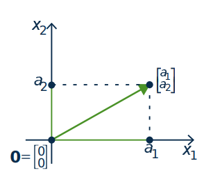
The set \(\mathbb{R}^2\) has a geometrical interpretation as the euclidean plane where a vector \(\left[ \begin{array}{c} a_{1} \\ a_{2} \end{array} \right]\) in \(\mathbb{R}^2\) represents the point \((a_{1}, a_{2})\) in the plane (see Figure [fig:003017]). In this way we regard \(\mathbb{R}^2\) as the set of all points in the plane. Accordingly, we will refer to vectors in \(\mathbb{R}^2\) as points, and denote their coordinates as a column rather than a row. To enhance this geometrical interpretation of the vector \(\left[ \begin{array}{c} a_{1} \\ a_{2} \end{array} \right]\), it is denoted graphically by an arrow from the origin \(\left[ \begin{array}{c} 0 \\ 0 \end{array} \right]\) to the vector as in Figure \(\PageIndex{2}\).

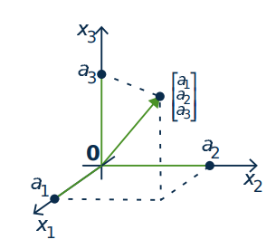
Similarly we identify \(\mathbb{R}^3\) with \(3\)-dimensional space by writing a point \((a_{1}, a_{2}, a_{3})\) as the vector \(\left[ \begin{array}{c} a_{1} \\ a_{2} \\ a_{3} \end{array} \right]\) in \(\mathbb{R}^3\), again represented by an arrow² from the origin to the point as in Figure [fig:003025]. In this way the terms “point” and “vector” mean the same thing in the plane or in space.

Figure \(\PageIndex{2}\):

Figure \(\PageIndex{3}\):

We begin by describing a particular geometrical transformation of the plane \(\mathbb{R}^2\).

Example \(\PageIndex{13}\)

Consider the transformation of \(\mathbb{R}^2\) given by reflection in the \(x\) axis. This operation carries the vector \(\left[ \begin{array}{c} a_{1} \\ a_{2} \end{array} \right]\) to its reflection \(\left[ \begin{array}{r} a_{1} \\ -a_{2} \end{array} \right]\) as in Figure [fig:003037]. Now observe that

Figure \(\PageIndex{4}\):

\[\left[ \begin{array}{r} a_{1} \\ -a_{2} \end{array} \right] = \left[ \begin{array}{rr} 1 & 0 \\ 0 & -1 \end{array} \right] \left[ \begin{array}{c} a_{1} \\ a_{2} \end{array} \right] \nonumber \]

so reflecting \(\left[ \begin{array}{c} a_{1} \\ a_{2} \end{array} \right]\) in the \(x\) axis can be achieved by multiplying by the matrix \(\left[ \begin{array}{rr} 1 & 0 \\ 0 & -1 \end{array} \right]\).

If we write \(A = \left[ \begin{array}{rr} 1 & 0 \\ 0 & -1 \end{array} \right]\), Example [exa:003028] shows that reflection in the \(x\) axis carries each vector \(\mathbf{x}\) in \(\mathbb{R}^2\) to the vector \(A\mathbf{x}\) in \(\mathbb{R}^2\). It is thus an example of a function

\[T : \mathbb{R}^{2} \to \mathbb{R}^{2} \quad \mbox{where} \quad T(\mathbf{x}) = A\mathbf{x} \mbox{ for all } \mathbf{x} \mbox{ in } \mathbb{R}^{2} \nonumber \]

As such it is a generalization of the familiar functions \(f : \mathbb{R} \to \mathbb{R}\) that carry a number \(x\) to another real number \(f(x)\).

Figure \(\PageIndex{5}\):

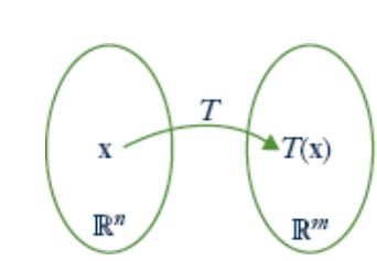
More generally, functions \(T : \mathbb{R}^n \to \mathbb{R}^m\) are called transformations from \(\mathbb{R}^n\) to \(\mathbb{R}^m\). Such a transformation \(T\) is a rule that assigns to every vector \(\mathbf{x}\) in \(\mathbb{R}^n\) a uniquely determined vector \(T(\mathbf{x})\) in \(\mathbb{R}^m\) called the image of \(\mathbf{x}\) under \(T\). We denote this state of affairs by writing

\[T : \mathbb{R}^{n} \to \mathbb{R}^{m} \quad \mbox{ or } \quad \mathbb{R}^{n} \xrightarrow{T} \mathbb{R}^{m} \nonumber \]

The transformation \(T\) can be visualized as in Figure [fig:003053].

To describe a transformation \(T : \mathbb{R}^n \to \mathbb{R}^m\) we must specify the vector \(T(\mathbf{x})\) in \(\mathbb{R}^m\) for every \(\mathbf{x}\) in \(\mathbb{R}^n\). This is referred to as defining \(T\), or as specifying the action of \(T\). Saying that the action defines the transformation means that we regard two transformations \(S : \mathbb{R}^n \to \mathbb{R}^m\) and \(T : \mathbb{R}^n \to \mathbb{R}^m\) as equal if they have the same action; more formally

\[S = T \quad \mbox{if and only if} \quad S(\mathbf{x}) = T(\mathbf{x}) \mbox{ for all } \mathbf{x} \mbox{ in } \mathbb{R}^{n}. \nonumber \]

Again, this what we mean by \(f = g\) where \(f, g : \mathbb{R} \to \mathbb{R}\) are ordinary functions.

Functions \(f : \mathbb{R} \to \mathbb{R}\) are often described by a formula, examples being \(f(x) = x^{2} + 1\) and \(f(x) = \sin x\). The same is true of transformations; here is an example.

Example \(\PageIndex{14}\)

The formula \(T \left[ \begin{array}{c} x_{1} \\ x_{2} \\ x_{3} \\ x_{4} \end{array} \right] = \left[ \begin{array}{c} x_{1} + x_{2} \\ x_{2} + x_{3} \\ x_{3} + x_{4} \end{array} \right]\) defines a transformation \(\mathbb{R}^4 \to \mathbb{R}^3\).

Example \(\PageIndex{13}\) suggests that matrix multiplication is an important way of defining transformations \(\mathbb{R}^n \to \mathbb{R}^m\). If \(A\) is any \(m \times n\) matrix, multiplication by \(A\) gives a transformation

\[T_{A} : \mathbb{R}^{n} \to \mathbb{R}^{m} \quad \mbox{defined by} \quad T_{A}(\mathbf{x}) = A\mathbf{x} \mbox{ for every } \mathbf{x} \mbox{ in } \mathbb{R}^{n} \nonumber \]

Definition: Matrix Transformation \(\PageIndex{5}\)

\(T_A\)003077 \(T_{A}\) is called the matrix transformation induced by \(A\).

Thus Example \(\PageIndex{13}\) shows that reflection in the x axis is the matrix transformation \(\mathbb{R}^2 \to \mathbb{R}^2\) induced by the matrix \(\left[ \begin{array}{rr} 1 & 0 \\ 0 & -1 \end{array} \right]\). Also, the transformation \(R : \mathbb{R}^4 \to \mathbb{R}^3\) in Example [exa:003028] is the matrix transformation induced by the matrix

\[A = \left[ \begin{array}{rrrr} 1 & 1 & 0 & 0 \\ 0 & 1 & 1 & 0 \\ 0 & 0 & 1 & 1 \\ \end{array} \right] \mbox{ because } \left[ \begin{array}{rrrr} 1 & 1 & 0 & 0 \\ 0 & 1 & 1 & 0 \\ 0 & 0 & 1 & 1 \\ \end{array} \right] \left[ \begin{array}{c} x_{1} \\ x_{2} \\ x_{3} \\ x_{4} \end{array} \right] = \left[ \begin{array}{c} x_{1} + x_{2} \\ x_{2} + x_{3} \\ x_{3} + x_{4} \end{array} \right] \nonumber \]

Example \(\PageIndex{15}\)

Let \(R_{\frac{\pi}{2}} : \mathbb{R}^{2} \to \mathbb{R}^{2}\) denote counterclockwise rotation about the origin through \(\frac{\pi}{2}\) radians (that is, \(90^{\circ}\)). Show that \(R_{\frac{\pi}{2}}\) is induced by the matrix \(\left[ \begin{array}{rr} 0 & -1 \\ 1 & 0 \end{array} \right]\).

Solution

Figure \(\PageIndex{6}\):

The effect of \(R_{\frac{\pi}{2}}\) is to rotate the vector \(\mathbf{x} = \left[ \begin{array}{c} a \\ b \end{array} \right]\) counterclockwise through \(\frac{\pi}{2}\) to produce the vector \(R_{\frac{\pi}{2}}(\mathbf{x})\) shown in Figure [fig:003108]. Since triangles \(\mathbf{0}\mathbf{p}\mathbf{x}\) and \(\mathbf{0}\mathbf{q}R_{\frac{\pi}{2}}(\mathbf{x})\) are identical, we obtain \(R_{\frac{\pi}{2}}(\mathbf{x}) = \left[ \begin{array}{r} -b \\ a \end{array} \right]\). But \(\left[ \begin{array}{r} -b \\ a \end{array} \right] = \left[ \begin{array}{rr} 0 & -1 \\ 1 & 0 \end{array} \right] \left[ \begin{array}{c} a \\ b \end{array} \right]\), so we obtain \(R_{\frac{\pi}{2}}(\mathbf{x}) = A\mathbf{x}\) for all \(\mathbf{x}\) in \(\mathbb{R}^2\) where \(A = \left[ \begin{array}{rr} 0 & -1 \\ 1 & 0 \end{array} \right]\). In other words, \(R_{\frac{\pi}{2}}\) is the matrix transformation induced by \(A\).

If \(A\) is the \(m \times n\) zero matrix, then \(A\) induces the transformation

\[T : \mathbb{R}^{n} \to \mathbb{R}^{m} \quad \mbox{given by} \quad T(\mathbf{x}) = A\mathbf{x} = \mathbf{0} \mbox{ for all } \mathbf{x} \mbox{ in } \mathbb{R}^{n} \nonumber \]

This is called the zero transformation, and is denoted \(T = 0\).

Another important example is the identity transformation

\[1_{\mathbb{R}^{n}} : \mathbb{R}^{n} \to \mathbb{R}^{n} \quad \mbox{ given by } \quad 1_{\mathbb{R}^{n}}(\mathbf{x}) = \mathbf{x} \mbox{ for all } \mathbf{x} \mbox{ in } \mathbb{R}^{n} \nonumber \]

That is, the action of \(1_{\mathbb{R}^n}\) on \(\mathbf{x}\) is to do nothing to it. If \(I_{n}\) denotes the \(n \times n\) identity matrix, we showed in Example [exa:002949] that \(I_{n} \mathbf{x} = \mathbf{x}\) for all \(\mathbf{x}\) in \(\mathbb{R}^n\). Hence \(1_{\mathbb{R}^n}(\mathbf{x}) = I_{n}\mathbf{x}\) for all \(\mathbf{x}\) in \(\mathbb{R}^n\); that is, the identity matrix \(I_{n}\) induces the identity transformation.

Here are two more examples of matrix transformations with a clear geometric description.

Example \(\PageIndex{16}\)

If \(a > 0\), the matrix transformation \(T \left[ \begin{array}{c} x \\ y \end{array} \right] = \left[ \begin{array}{c} ax \\ y \end{array} \right]\) induced by the matrix \(A = \left[ \begin{array}{cc} a & 0 \\ 0 & 1 \end{array} \right]\) is called an \(\boldsymbol{x}\)-expansion of \(\mathbb{R}^2\) if \(a > 1\), and an \(\boldsymbol{x}\)-compression if \(0 < a < 1\). The reason for the names is clear in the diagram below. Similarly, if \(b > 0\) the matrix \(A = \left[ \begin{array}{cc} 1 & 0 \\ 0 & b \end{array} \right]\) gives rise to \(\boldsymbol{y}\)-expansions and \(\boldsymbol{y}\)-compressions.

Figure \(\PageIndex{7}\):

Example \(\PageIndex{17}\)

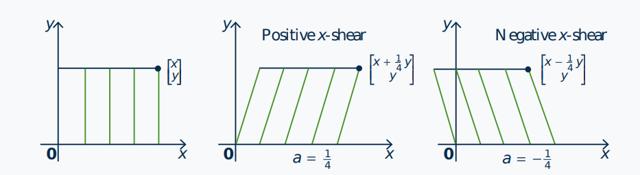
If \(a\) is a number, the matrix transformation \(T \left[ \begin{array}{c} x \\ y \end{array} \right] = \left[ \begin{array}{c} x + ay \\ y \end{array} \right]\) induced by the matrix \(A = \left[ \begin{array}{cc} 1 & a \\ 0 & 1 \end{array} \right]\) is called an \(\boldsymbol{x}\)-shear of \(\mathbb{R}^2\) (positive if \(a > 0\) and negative if \(a < 0)\). Its effect is illustrated below when \(a = \frac{1}{4}\) and \(a = -\frac{1}{4}\).

Figure \(\PageIndex{8}\):

We hasten to note that there are important geometric transformations that are not matrix transformations. For example, if \(\mathbf{w}\) is a fixed column in \(\mathbb{R}^n\), define the transformation \(T_{\mathbf{w}} : \mathbb{R}^n \to \mathbb{R}^n\) by

\[T_{\mathbf{w}}(\mathbf{x}) = \mathbf{x} + \mathbf{w} \quad \mbox{ for all } \mathbf{x} \mbox{ in } \mathbb{R}^{n} \nonumber \]

Then \(T_{\mathbf{w}}\) is called translation by \(\mathbf{w}\). In particular, if \(\mathbf{w} = \left[ \begin{array}{r} 2 \\ 1 \end{array} \right]\) in \(\mathbb{R}^2\), the effect of \(T_{\mathbf{w}}\) on \(\left[ \begin{array}{c} x \\ y \end{array} \right]\) is to translate it two units to the right and one unit up (see Figure \(\PageIndex{9}\)).

Figure \(\PageIndex{9}\):

The translation \(T_{\mathbf{w}}\) is not a matrix transformation unless \(\mathbf{w} = \mathbf{0}\). Indeed, if \(T_{\mathbf{w}}\) were induced by a matrix \(A\), then \(A\mathbf{x} = T_{\mathbf{w}}(\mathbf{x}) = \mathbf{x} + \mathbf{w}\) would hold for every \(\mathbf{x}\) in \(\mathbb{R}^n\). In particular, taking \(\mathbf{x} = \mathbf{0}\) gives \(\mathbf{w} = A\mathbf{0} = \mathbf{0}\).

---

1. Linear combinations were introduced in Section [sec:1_3] to describe the solutions of homogeneous systems of linear equations. They will be used extensively in what follows.↩
2. This “arrow” representation of vectors in \(\mathbb{R}^2\) and \(\mathbb{R}^3\) will be used extensively in Chapter [chap:4].↩