4.4: Vectors, Lists and Functions- \(\mathbb{R}^{S}\)

Suppose you are going shopping. You might jot down something like this on a piece of paper:

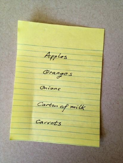
We could represent this information mathematically as a set, $$S=\{\rm apple, orange, onion, milk, carrot\}\, .\]

There is no information of ordering here and no information about how many carrots you will buy. This set by itself is not a vector; how would we add such sets to one another?

If you were a more careful shopper your list might look like this:

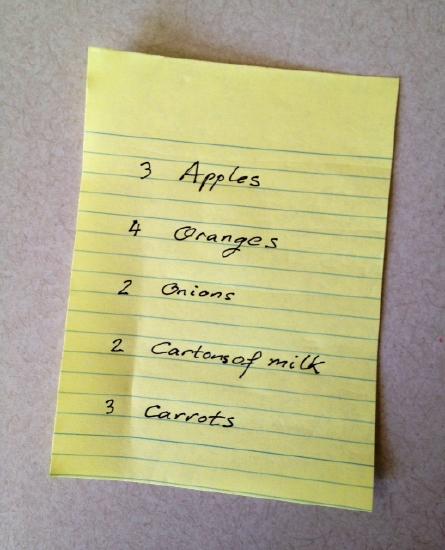
What you have really done here is assign a number to each element of the set \(S\). In other words, the second list is a function
$$
f:S\longrightarrow {\mathbb R}\, .
$$
Given two lists like the second one above, we could easily add them -- if you plan to buy 5 apples and I am buying 3 apples, together we will buy 8 apples! In fact, the second list is really a 5-vector in disguise.

In general it is helpful to think of an \(n\)-vector as a function whose domain is the set \(\{1,\dots,n\}\). This is equivalent to thinking of an \(n\)-vector as an ordered list of \(n\) numbers. These two ideas give us two equivalent notions for the set of all \(n\)-vectors:
$$
{\mathbb{R}}^{n} :=\left\{ \begin{pmatrix}a^{1} \\ \vdots \\ a^{n}\end{pmatrix} \middle\vert \, a^{1},\dots a^{n} \in \mathbb{R} \right\}
=\{ a:\{1,\dots,n\}\to \mathbb{R}\} := \mathbb{R}^{ \{1,\cdots,n\} }
$$
The notation \(\mathbb{R}^{ \{1,\cdots,n\} }\) is used to denote functions from \(\{1,\dots,n\}\) to \(\mathbb{R}\). Similarly, for any set \(S\) the notation \(\mathbb{R}^{S}\) denotes the set of functions from \(S\) to \(\mathbb{R}\):
$$
\mathbb{R}^{S}:=\{ f:S\to \mathbb {R}\}\, .
$$
When \(S\) is an ordered set like \(\{1,\dots,n\}\), it is natural to write the components in order. When the elements of \(S\) do not have a natural ordering, doing so might cause confusion.

Example \(\PageIndex{1}\):

Consider the set \(S=\{*, \star, \# \}\) from chapter 1 review problem 9. A particular element of \(\mathbb{R}^{S}\) is the function \(a\) explicitly defined by
$$ a^{\star}=3, a^{\#}=5, a^{*}=-2.$$
It is not natural to write
$$
a=\begin{pmatrix}3 \\ 5 \\ -2\end{pmatrix} ~{\rm or} ~a=\begin{pmatrix}-2\\ 3 \\ 5\end{pmatrix}
$$
because the elements of \(S\) do not have an ordering, since as sets \(\{*, \star, \# \}=\{*,\star,\#\}\).

In this important way, \(\mathbb{R}^{S}\) seems different from \(\mathbb{R}^{3}\). What is more evident are the similarities; since we can add two functions, we can add two elements of \(\mathbb{R}^{S}\):

Addition in \(\mathbb{R}^{S}\)

If \(a^{\star}=3, a^{\#}=5, a^{*}=-2\) and \(b^{\star}=-2, b^{\#}=4, b^{*}=13\)
then \(a+b\) is the function
$$(a+b)^{\star}=3-2=1, (a+b)^{\#}=5+4=9, (a+b)^{*}=-2+13=11\, .\]

Also, since we can multiply functions by numbers, there is a notion of scalar multiplication on \(\mathbb{R}^{S}\):

Scalar Multiplication in \(\mathbb{R}^{S}\)

If \(a^{\star}=3, a^{\#}=5, a^{*}=-2\),
then \(3a\) is the function
$$(3a)^{\star}=3\cdot3=9, (3a)^{\#}=3\cdot5=15, (3a)^{*}=3(-2)=-6\, .\]

We visualize \(\mathbb{R}^{2}\) and \(\mathbb{R}^{3}\) in terms of axes. We have a more abstract picture of \(\mathbb{R}^{4}\), \(\mathbb{R}^{5}\) and \(\mathbb{R}^{n}\) for larger \(n\) while \(\mathbb{R}^{S}\) seems even more abstract. However, when thought of as a simple "shopping list'', you can see that vectors in \(\mathbb{R}^{S}\) in fact, can describe everyday objects. In chapter 5 we introduce the general definition of a vector space that unifies all these different notions of a vector.

Contributor

• David Cherney, Tom Denton, and Andrew Waldron (UC Davis)