12.1: Invariant Directions

Have a look at the linear transformation \(L\) depicted below:

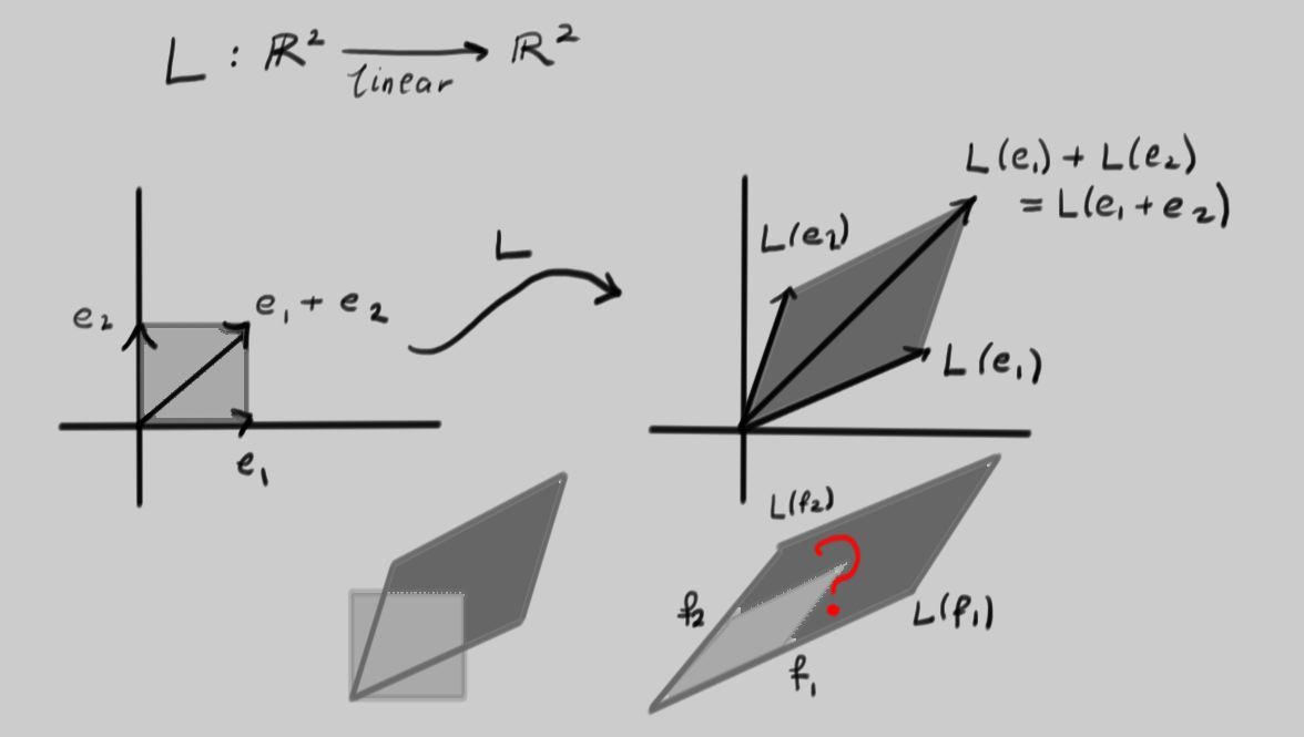
It was picked at random by choosing a pair of vectors \(L(e_{1})\) and \(L(e_{2})\) as the outputs of \(L\) acting on the canonical basis vectors. Notice how the unit square with a corner at the origin is mapped to a parallelogram. The second line of the picture shows these superimposed on one another. Now look at the second picture on that line. There, two vectors \(f_{1}\) and \(f_{2}\) have been carefully chosen such that if the inputs into \(L\) are in the parallelogram spanned by \(f_{1}\) and \(f_{2}\), the outputs also form a parallelogram with edges lying along the same two directions. Clearly this is a very special situation that should correspond to interesting properties of \(L\).

Now lets try an explicit example to see if we can achieve the last picture:

Example 116

Consider the linear transformation \(L\) such that $$L\begin{pmatrix}1\\0\end{pmatrix}=\begin{pmatrix}-4\\-10\end{pmatrix}\, \mbox{ and }\, L\begin{pmatrix}0\\1\end{pmatrix}=\begin{pmatrix}3\\7\end{pmatrix}\, ,$$ so that the matrix of \(L\) is

\[\begin{pmatrix}
-4 & 3 \\
-10 & 7 \\
\end{pmatrix}\, .\]

Recall that a vector is a direction and a magnitude; \(L\) applied to \(\begin{pmatrix}1\\0\end{pmatrix}\) or \(\begin{pmatrix}0\\1\end{pmatrix}\) changes both the direction and the magnitude of the vectors given to it.

Notice that $$L\begin{pmatrix}3\\5\end{pmatrix}=\begin{pmatrix}-4\cdot 3+3\cdot 5 \\ -10\cdot 3+7\cdot 5\end{pmatrix}=\begin{pmatrix}3\\5\end{pmatrix}\, .$$ Then \(L\) fixes the direction (and actually also the magnitude) of the vector \(v_{1}=\begin{pmatrix}3\\5\end{pmatrix}\).

Now, notice that any vector with the same direction as \(v_{1}\) can be written as \(cv_{1}\) for some constant \(c\). Then \(L(cv_{1})=cL(v_{1})=cv_{1}\), so \(L\) fixes every vector pointing in the same direction as \(v_{1}\).

Also notice that

\[L\begin{pmatrix}1\\2\end{pmatrix}=\begin{pmatrix}-4\cdot 1+3\cdot 2 \\ -10\cdot 1+7\cdot 2\end{pmatrix}=\begin{pmatrix}2\\4\end{pmatrix}=2\begin{pmatrix}1\\2\end{pmatrix}\, ,\]

so \(L\) fixes the direction of the vector \(v_{2}=\begin{pmatrix}1\\2\end{pmatrix}\) but stretches \(v_{2}\) by a factor of \(2\). Now notice that for any constant \(c\), \(L(cv_{2})=cL(v_{2})=2cv_{2}\). Then \(L\) stretches every vector pointing in the same direction as \(v_{2}\) by a factor of \(2\).

In short, given a linear transformation \(L\) it is sometimes possible to find a vector \(v\neq 0\) and constant \(\lambda\neq 0\) such that \(Lv=\lambda v.\)

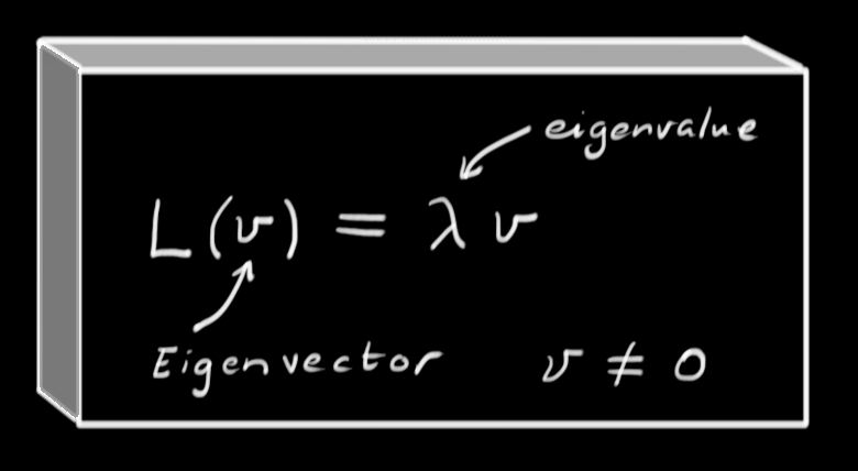
We call the direction of the vector \(v\) an \(\textit{invariant direction}\). In fact, any vector pointing in the same direction also satisfies this equation because \(L(cv)=cL(v)=\lambda cv\). More generally, any \(\textit{non-zero}\) vector \(v\) that solves

\[Lv=\lambda v\]

is called an \(\textit{eigenvector}\) of \(L\), and \(\lambda\) (which now need not be zero) is an \(\textit{eigenvalue}\). Since the direction is all we really care about here, then any other vector \(cv\) (so long as \(c\neq 0\)) is an equally good choice of eigenvector. Notice that the relation "\(u\) and \(v\) point in the same direction'' is an equivalence relation.

In our example of the linear transformation \(L\) with matrix

\[\begin{pmatrix}
-4 & 3 \\
-10 & 7 \\
\end{pmatrix}\, ,\]

we have seen that \(L\) enjoys the property of having two invariant directions, represented by eigenvectors \(v_{1}\) and \(v_{2}\) with eigenvalues \(1\) and \(2\), respectively.

It would be very convenient if we could write any vector \(w\) as a linear combination of \(v_{1}\) and \(v_{2}\). Suppose \(w=rv_{1}+sv_{2}\) for some constants \(r\) and \(s\). Then:

\[L(w)=L(rv_{1}+sv_{2})=rL(v_{1})+sL(v_{2})=rv_{1}+2sv_{2}.\]

Now \(L\) just multiplies the number \(r\) by \(1\) and the number \(s\) by \(2\). If we could write this as a matrix, it would look like:

\[
\begin{pmatrix}
1 & 0 \\
0 & 2
\end{pmatrix}\begin{pmatrix}s\\t\end{pmatrix}
\]

which is much slicker than the usual scenario

\[L\!\begin{pmatrix}
x\\
y
\end{pmatrix}\!=\!\begin{pmatrix}
\!a&b\! \\
\!c&d\!
\end{pmatrix} \! \!\begin{pmatrix}
x \\
y
\end{pmatrix}\!=\!
\begin{pmatrix}
\!ax+by\! \\
\!cx+dy\!
\end{pmatrix}\, .\]

Here, \(s\) and \(t\) give the coordinates of \(w\) in terms of the vectors \(v_{1}\) and \(v_{2}\). In the previous example, we multiplied the vector by the matrix \(L\) and came up with a complicated expression. In these coordinates, we see that \(L\) has a very simple diagonal matrix, whose diagonal entries are exactly the eigenvalues of \(L\).

This process is called diagonalization. It makes complicated linear systems much easier to analyze.

Now that we've seen what eigenvalues and eigenvectors are, there are a number of questions that need to be answered.

1. How do we find eigenvectors and their eigenvalues?
2. How many eigenvalues and (independent) eigenvectors does a given linear transformation have?
3. When can a linear transformation be diagonalized?

We'll start by trying to find the eigenvectors for a linear transformation.

Example 117

Let \(L \colon \Re^{2}\rightarrow \Re^{2}\) such that \(L(x,y)=(2x+2y, 16x+6y)\). First, we find the matrix of \(L\):

\[\begin{pmatrix}x\\y\end{pmatrix}\stackrel{L}{\longmapsto} \begin{pmatrix}
2 & 2 \\
16 & 6
\end{pmatrix}\begin{pmatrix}x\\y\end{pmatrix}.\]

We want to find an invariant direction \(v=\begin{pmatrix}x\\y\end{pmatrix}\) such that

\[Lv=\lambda v\]

or, in matrix notation,
\begin{equation*}
\begin{array}{lrcl}
&\begin{pmatrix}
2 & 2 \\
16 & 6
\end{pmatrix}\begin{pmatrix}x\\y\end{pmatrix}&=&\lambda \begin{pmatrix}x\\y\end{pmatrix} \\
\Leftrightarrow &\begin{pmatrix}
2 & 2 \\
16 & 6
\end{pmatrix}\begin{pmatrix}x\\y\end{pmatrix}&=&\begin{pmatrix}
\lambda & 0 \\
0 & \lambda
\end{pmatrix} \begin{pmatrix}x\\y\end{pmatrix} \\
\Leftrightarrow& \begin{pmatrix}
2-\lambda & 2 \\
16 & 6-\lambda
\end{pmatrix}\begin{pmatrix}x\\y\end{pmatrix}&=& \begin{pmatrix}0\\0\end{pmatrix}\, .
\end{array}
\end{equation*}
This is a homogeneous system, so it only has solutions when the matrix \(\begin{pmatrix}
2-\lambda & 2 \\
16 & 6-\lambda
\end{pmatrix}\) is singular. In other words,
\begin{equation*}
\begin{array}{lrcl}
&\det \begin{pmatrix}
2-\lambda & 2 \\
16 & 6-\lambda
\end{pmatrix}&=&0 \\
\Leftrightarrow& (2-\lambda)(6-\lambda)-32&=&0 \\
\Leftrightarrow &\lambda^{2}-8\lambda-20&=&0\\
\Leftrightarrow &(\lambda-10)(\lambda+2)&=&0
\end{array}
\end{equation*}

For any square \(n\times n\) matrix \(M\), the polynomial in \(\lambda\) given by $$P_{M}(\lambda)=\det (\lambda I-M)=(-1)^{n} \det (M-\lambda I)$$ is called the \(\textit{characteristic polynomial}\) of \(M\), and its roots are the eigenvalues of \(M\).

In this case, we see that \(L\) has two eigenvalues, \(\lambda_{1}=10\) and \(\lambda_{2}=-2\). To find the eigenvectors, we need to deal with these two cases separately. To do so, we solve the linear system \(\begin{pmatrix}
2-\lambda & 2 \\
16 & 6-\lambda
\end{pmatrix}\begin{pmatrix}x\\y\end{pmatrix}= \begin{pmatrix}0\\0\end{pmatrix}\) with the particular eigenvalue \(\lambda\) plugged in to the matrix.

1. [\(\underline{\lambda=10}\):] We solve the linear system

\[\begin{pmatrix}
-8 & 2 \\
16 & -4
\end{pmatrix}\begin{pmatrix}x\\y\end{pmatrix}= \begin{pmatrix}0\\0\end{pmatrix}.
\]
Both equations say that \(y=4x\), so any vector \(\begin{pmatrix}x\\4x\end{pmatrix}\) will do. Since we only need the direction of the eigenvector, we can pick a value for \(x\). Setting \(x=1\) is convenient, and gives the eigenvector \(v_{1}=\begin{pmatrix}1\\4\end{pmatrix}\).

2. [\(\underline{\lambda=-2}\):] We solve the linear system

\[\begin{pmatrix}
4 & 2 \\
16 & 8
\end{pmatrix}\begin{pmatrix}x\\y\end{pmatrix}= \begin{pmatrix}0\\0\end{pmatrix}.
\]
Here again both equations agree, because we chose \(\lambda\) to make the system singular. We see that \(y=-2x\) works, so we can choose \(v_{2}=\begin{pmatrix}1\\-2\end{pmatrix}\).

Our process was the following:

1. Find the characteristic polynomial of the matrix \(M\) for \(L\), given by \(\det (\lambda I-M)\).
2. Find the roots of the characteristic polynomial; these are the eigenvalues of \(L\).
3. For each eigenvalue \(\lambda_{i}\), solve the linear system \((M-\lambda_{i} I)v=0\) to obtain an eigenvector \(v\) associated to \(\lambda_{i}\).

Contributor

• David Cherney, Tom Denton, and Andrew Waldron (UC Davis)