18.10: Movie Scripts 7-8

G.7 Determinants

Permutation Example

Lets try to get the hang of permutations. A permutation is a function which scrambles things. Suppose we had

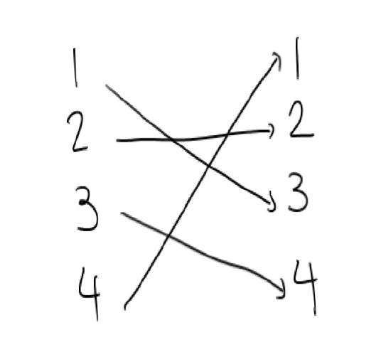
This looks like a function $\sigma$ that has values $$\sigma(1) =3 ,\ \sigma(2) =2 ,\ \sigma(3) =4 ,\ \sigma(4) = 1\, .$$

Then we could write this as
$$\begin{bmatrix} 1 & 2 & 3 & 4\\ \sigma(1) & \sigma(2) & \sigma(3) & \sigma(4) \end{bmatrix} = \begin{bmatrix} 1 & 2 & 3 & 4 \\ 3 & 2 & 4 & 1 \end{bmatrix}$$
We could write this permutation in two steps by saying that first we swap 3 and 4, and then we swap 1 and 3. The order here is important.

This is an even permutation, since the number of swaps we used is two (an even number).

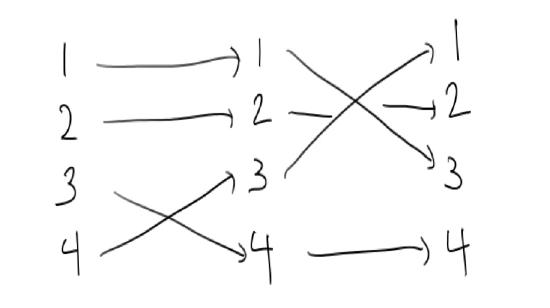
Elementary Matrices

This video will explain some of the ideas behind elementary matrices. First think back to linear systems, for example $n$ equations in $n$ unknowns:
$$\left\{ \begin{array}{ccc} a^{1}_{1} x^{1} + a^{1}_{2} x^{2}+\cdots +a^{1}_{n} x^{n} &=&v^{1}\\ a^{2}_{1} x^{1} + a^{2}_{2} x^{2}+\cdots +a^{2}_{n} x^{n} &=&v^{2}\\ \vdots &&\\ a^{n}_{1} x^{1} + a^{n}_{2} x^{2}+\cdots +a^{n}_{n} x^{n} &=&v^{n}\, . \end{array}\right .$$
We know it is helpful to store the above information with matrices and vectors
$$M:=\begin{pmatrix} a^{1}_{1}&a^{1}_{2}&\cdots& a^{1}_{n}\\ a^{2}_{1}&a^{2}_{2}&\cdots& a^{2}_{n}\\ \vdots&\vdots&&\vdots\\ a^{n}_{1}&a^{n}_{2}&\cdots& a^{n}_{n}\\ \end{pmatrix}\, ,\qquad X:=\begin{pmatrix}x^{1}\\x^{2}\\\vdots\\ x^{n}\end{pmatrix}\, ,\qquad V:=\begin{pmatrix}v^{1}\\v^{2}\\\vdots\\v^{n}\end{pmatrix}\, .$$
Here we will focus on the case the $M$ is square because we are interested in its inverse $M^{-1}$ (if it exists) and its determinant (whose job it will be to determine the existence of $M^{-1}$).

We know at least three ways of handling this linear system problem:

1. As an augmented matrix $$\left(\begin{array}{c|c}M & V\end{array}\right)\, .$$ Here our plan would be to perform row operations until the system looks like $$\left(\begin{array}{c|c}I & M^{-1}V\end{array}\right)\, ,$$ (assuming that $M^{-1}$ exists).
2. As a matrix equation $$MX=V\, ,$$ which we would solve by finding $M^{-1}$ (again, if it exists), so that $$X=M^{-1}V\, .$$
3. As a linear transformation $$L:\mathbb{R}^{n}\longrightarrow \mathbb{R}^{n}$$ via $$\mathbb{R}^{n}\ni X \longmapsto MX \in \mathbb{R}^{n}\, .$$ In this case we have to study the equation $L(X)=V$ because $V\in \mathbb{R}^{n}$.

Lets focus on the first two methods. In particular we want to think about how the augmented matrix method can give information about finding $M^{-1}$. In particular, how it can be used for handling determinants.

The main idea is that the row operations changed the augmented matrices, but we also know how to change a matrix $M$ by multiplying it by some other matrix $E$, so that $M\to EM$. In particular can we find ``elementary matrices'' the perform row operations?

Once we find these elementary matrices is is $\textit{very important}$ to ask how they effect the determinant, but you can think about that for your own self right now.

Lets tabulate our names for the matrices that perform the various row operations:
$$\left( $$\begin{array}{r|r} Row Operation & Elementary Matrix \\ \hline R_{i}\leftrightarrow R_{j} & E_{j}^{i} \\ R_{i} \to \lambda R_{i} & R^{i}(\lambda) \\ R_{i} \to R_{i} + \lambda R_{j} & S^{i}_{j}(\lambda)\end{array}$$ \right)\]

To finish off the video, here is how all these elementary matrices work for a $2\times 2$ example. Lets take
$$M=\begin{pmatrix}a&b\\c&d\end{pmatrix}\, .$$
A good thing to think about is what happens to $\det M = ad-bc$ under the operations below.

1. Row swap: $$E^{1}_{2}=\begin{pmatrix}0&1\\1&0\end{pmatrix}\, ,\qquad E^{1}_{2} M = \begin{pmatrix}0&1\\1&0\end{pmatrix}\begin{pmatrix}a&b\\c&d\end{pmatrix}=\begin{pmatrix}c&d\\a&b\end{pmatrix}\, .$$
2. Scalar multiplying: $$R^{1}(\lambda)=\begin{pmatrix}\lambda&0\\0&1\end{pmatrix}\, ,\qquad E^{1}_{2} M = \begin{pmatrix}\lambda&0\\0&1\end{pmatrix}\begin{pmatrix}a&b\\c&d\end{pmatrix}=\begin{pmatrix}\lambda a&\lambda b\\c&d\end{pmatrix}\, .$$
3. Row sum: $$S^{1}_{2}(\lambda)=\begin{pmatrix}1&\lambda\\0&1\end{pmatrix}\, ,\quad S^{1}_{2}(\lambda) M = \begin{pmatrix}1&\lambda\\0&1\end{pmatrix}\begin{pmatrix}a&b\\c&d\end{pmatrix}=\begin{pmatrix}a+\lambda c&b+\lambda d\\c&d\end{pmatrix}\, .$$

Elementary Determinants

This video will show you how to calculate determinants of elementary matrices. First remember that the job of an elementary row matrix is to perform row operations, so that if $E$ is an elementary row matrix and $M$ some given matrix, $$EM$$ is the matrix $M$ with a row operation performed on it.

The next thing to remember is that the determinant of the identity is $1$. Moreover, we also know what row operations do to determinants:

1. Row swap $E^{i}_{j}$: flips the sign of the determinant.
2. Scalar multiplication $R^{i}(\lambda)$: multiplying a row by $\lambda$ multiplies the determinant by $\lambda$.
3. Row addition $S^{i}_{j}(\lambda)$: adding some amount of one row to another does not change the determinant.

The corresponding elementary matrices are obtained by performing exactly these operations on the identity:
$$
E^{i}_{j}= $$\begin{pmatrix} 1 & & & & & & \\ & \ddots & & & & & \\ & & 0 & & 1 & & \\ & & & \ddots & & & \\ & & 1 & & 0 & & \\ & & & & & \ddots& \\ & & & & & & 1 \\ \end{pmatrix}$$ \, ,
\]

$$R^{i}(\lambda)= \begin{pmatrix} 1 & & & & \\ & \ddots & & & \\ & & \lambda & & \\ & & & \ddots & \\ & & & & 1 \\ \end{pmatrix} \, ,$$

$$S^{i}_{j}(\lambda) = \begin{pmatrix} 1 & & & & & & \\ & \ddots & & & & & \\ & & 1 & & \lambda & & \\ & & & \ddots & & & \\ & & & & 1 & & \\ & & & & & \ddots& \\ & & & & & & 1 \\ \end{pmatrix}$$
So to calculate their determinants, we just have to apply the above list of what happens to the determinant of a matrix under row operations to the determinant of the identity. This yields
$$
\det E^{i}_{j}=-1\, ,\qquad
\det R^{i}(\lambda)=\lambda\, ,\qquad
\det S^{i}_{j}(\lambda)=1\, .
\]

Determinants and Inverses

Lets figure out the relationship between determinants and invertibility. If we have a system of equations $Mx=b$ and we have the inverse $M^{-1}$ then if we multiply on both sides we get $x = M^{-1}Mx= M^{-1}b$. If the inverse exists we can solve for $x$ and get a solution that looks like a point.

So what could go wrong when we want solve a system of equations and get a solution that looks like a point? Something would go wrong if we didn't have enough equations for example if we were just given
$$x+y = 1$$
or maybe, to make this a square matrix $M$ we could write this as
$$\begin{align*} x+y &= 1\\ 0 &= 0 \end{align*}$$
The matrix for this would be
$M =\begin{bmatrix} 1 & 1\\ 0& 0 \end{bmatrix}$
and det$(M) = 0$. When we compute the determinant, this row of all zeros gets multiplied in every term. If instead we were given redundant equations

$$\begin{align*} x+y &= 1\\ 2x+2y &= 2 \end{align*}$$
The matrix for this would be
$M =\begin{bmatrix} 1 & 1\\ 2& 2 \end{bmatrix}$ and det$(M) = 0$. But we know that with an elementary row operation, we could replace the second row with a row of all zeros. Somehow the determinant is able to detect that there is only one equation here. Even if we had a set of contradictory set of equations such as
$$\begin{align*} x+y &= 1\\ 2x+2y &= 0, \end{align*}$$
where it is not possible for both of these equations to be true, the matrix $M$ is still the same, and still has a determinant zero.

Lets look at a three by three example, where the third equation is the sum of the first two equations.

$$\begin{align*} x+y + z &= 1\\ y +z &= 1\\ x + 2y+ 2z &= 2\\ \end{align*}$$

and the matrix for this is

$$M =\begin{bmatrix} 1 & 1 &1\\ 0 & 1 & 1\\ 1 & 2& 2 \end{bmatrix}$$

If we were trying to find the inverse to this matrix using elementary matrices
$$\left( \begin{array}{ccc | ccc} 1 & 1 &1 & 1 & 0 & 0\\ 0 & 1 & 1 & 0 & 1 & 0 \\ 1 & 2 & 2 & 0 & 0 & 1 \end{array} \right) = \left( \begin{array}{ccc | rrr} 1 & 1 &1 & 1 & 0 & 0\\ 0 & 1 & 1 & 0 & 1 & 0 \\ 0 & 0 & 0 & -1 & -1 & 1 \end{array} \right)$$
And we would be stuck here. The last row of all zeros cannot be converted into the bottom row of a $3 \times 3$ identity matrix. this matrix has no inverse, and the row of all zeros ensures that the determinant will be zero. It can be difficult to see when one of the rows of a matrix is a linear combination of the others, and what makes the determinant a useful tool is that with this reasonably simple computation we can find out if the matrix is invertible, and if the system will have a solution of a single point or column vector.

Alternative Proof

Here we will prove more directly that} the determinant of a product of matrices is the product of their determinants. First we reference that for a matrix $M$ with rows $r_{i}$, if $M^{\prime}$ is the matrix with rows $r^{\prime}_{j} = r_{j} + \lambda r_{i}$ for $j \neq i$ and $r^{\prime}_{i} = r_{i}$, then $\det(M) = \det(M^{\prime})$. Essentially we have $M^{\prime}$ as $M$ multiplied by the elementary row sum matrices $S^{i}_{j}(\lambda)$. Hence we can create an upper-triangular matrix $U$ such that $\det(M) = \det(U)$ by first using the first row to set $m_{i}^{1} \mapsto 0$ for all $i > 1$, then iteratively (increasing $k$ by 1 each time) for fixed $k$ using the $k$-th row to set $m_{i}^{k} \mapsto 0$ for all $i > k$.

Now note that for two upper-triangular matrices $U = (u_{i}^{j})$ and $U^{\prime} = (u_{i}^{\prime j})$, by matrix multiplication we have $X = UU^{\prime} = (x_{i}^{j})$ is upper-triangular and $x_{i}^{i} = u_{i}^{i} u_{i}^{\prime i}$. Also since every permutation would contain a lower diagonal entry (which is 0) have $\det(U) = \prod_{i} u_{i}^{i}$. Let $A$ and $A^{\prime}$ have corresponding upper-triangular matrices $U$ and $U^{\prime}$ respectively (i.e. $\det(A) = \det(U)$), we note that $AA^{\prime}$ has a corresponding upper-triangular matrix $UU^{\prime}$, and hence we have
$$\begin{align*} \det(A A^{\prime}) & = \det(U U^{\prime}) = \prod_{i} u_{i}^{i} u_{i}^{\prime i} \\ & = \left( \prod_{i} u_{i}^{i} \right) \left( \prod_{i} u_{i}^{\prime i} \right) \\ & = \det(U) \det(U^{\prime}) = \det(A) \det(A^{\prime}). \end{align*}$$

Practice taking Determinants

Lets practice taking determinants of $2 \times 2$ and $3\times 3$ matrices.

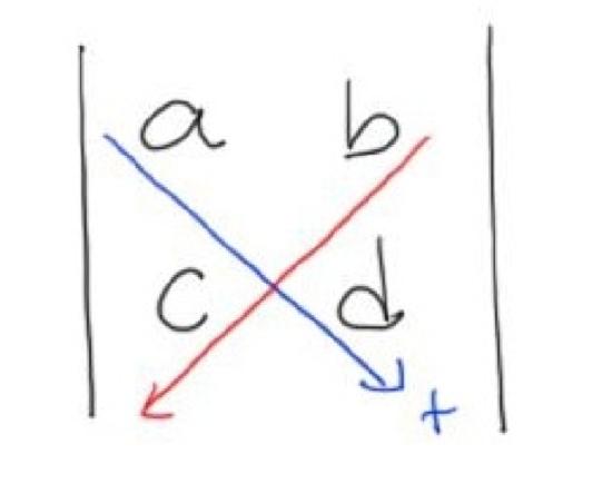
For $2 \times 2$ matrices we have a formula
$${\rm det} \begin{pmatrix} a & b \\ c & d \\ \end{pmatrix} = ad - bc\, .$$
This formula might be easier to remember if you think about this picture.

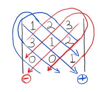
Now we can look at three by three matrices and see a few ways to compute the determinant. We have a similar pattern for $3\times 3$ matrices.
Consider the example
$${\rm det} \begin{pmatrix} 1 & 2 & 3 \\ 3 & 1 & 2 \\ 0 & 0 & 1 \\ \end{pmatrix} = ( (1\cdot 1\cdot 1)+ (2\cdot 2\cdot 0) + (3\cdot 3\cdot 0)) - ((3\cdot 1\cdot 0)+ (1\cdot 2\cdot 0) + (3\cdot 2\cdot 1)) = -5$$
We can draw a picture with similar diagonals to find the terms that will be positive and the terms that will be negative.

Another way to compute the determinant of a matrix is to use this recursive formula. Here I take the coefficients of the first row and multiply them by the determinant of the minors and the cofactor. Then we can use the formula for a two by two determinant to compute the determinant of the minors

$$\text{det} \begin{pmatrix} 1 & 2 & 3 \\ 3 & 1 & 2 \\ 0 & 0 & 1 \\ \end{pmatrix} = 1 \begin{vmatrix} 1 & 2 \\ 0 &1\\ \end{vmatrix} -2 \begin{vmatrix} 3 & 2 \\ 0 & 1 \\ \end{vmatrix} + 3 \begin{vmatrix} 3 & 1 \\ 0 & 0 \\ \end{vmatrix}\\ = 1(1-0) - 2(3-0) + 3(0-0) = -5$$
Decide which way you prefer and get good at taking determinants, you'll need to compute them in a lot of problems.

Hint for Review Problem 5

For an arbitrary $3 \times 3$ matrix $A = (a^{i}_{j})$, we have
$$\det(A) = a^{1}_{1} a^{2}_{2} a^{3}_{3} + a^{1}_{2} a^{2}_{3} a^{3}_{1} + a^{1}_{3} a^{2}_{1} a^{3}_{2} - a^{1}_{1} a^{2}_{3} a^{3}_{2} - a^{1}_{2} a^{2}_{1} a^{3}_{3} - a^{1}_{3} a^{2}_{2} a^{3}_{1}$$
and so the complexity is $5a + 12m$. Now note that in general, the complexity $c_{n}$ of the expansion minors formula of an arbitrary $n \times n$ matrix should be
$$c_{n} = (n-1) a + n c_{n-1} m$$
since $\det(A) = \sum_{i=1}^{n} (-1)^{i} a_{i}^{1} cofactor(a_{i}^{1})$ and $cofactor(a_{i}^{1})$ is an $(n-1) \times (n-1)$ matrix. This is one way to prove part (c).

G.8 Subspaces and Spanning Sets

Linear Systems as Spanning Sets

Suppose that we were given a set of linear equations $l^{j}(x^{1}, x^{2}, \dotsc, x^{n})$ and we want to find out if $l^{j}(X) = v^{j}$ for all $j$ for some vector $V = (v^{j})$. We know that we can express this as the matrix equation
$$\sum_{i} l^{j}_{i} x^{i} = v^{j}$$
where $l^{j}_{i}$ is the coefficient of the variable $x^{i}$ in the equation $l^{j}$. However, this is also stating that $V$ is in the span of the vectors $\{ L_{i} \}_{i}$ where $L_{i} = (l^{j}_{i})_{j}$. For example, consider the set of equations
$$\begin{align*} 2 x + 3 y - z & = 5 \\ -x + 3y + z & = 1 \\ x + y - 2 z & = 3 \end{align*}$$
which corresponds to the matrix equation
$$\begin{pmatrix} 2 & 3 & -1 \\ -1 & 3 & 1 \\ 1 & 1 & -2 \end{pmatrix} \begin{pmatrix} x \\ y \\ z \end{pmatrix} = \begin{pmatrix} 5 \\ 1 \\ 3 \end{pmatrix}.$$
We can thus express this problem as determining if the vector
$$V = \begin{pmatrix} 5 \\ 1 \\ 3 \end{pmatrix}$$
lies in the span of
$$\left\{ \begin{pmatrix} 2 \\ -1 \\ 1 \end{pmatrix}, \begin{pmatrix} 3 \\ 3 \\ 1 \end{pmatrix}, \begin{pmatrix} -1 \\ 1 \\ -2 \end{pmatrix} \right\}.$$

Hint for Review Problem 2

For the first part, try drawing an example in $\mathbb{R}^{3}$:

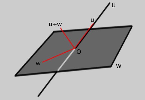
Here we have taken the subspace $W$ to be a plane through the origin and $U$ to be a line through the origin. The hint now is to think about what happens when you add a vector $u\in U$ to a vector $w\in W$. Does this live in the union $U\cup W$?

For the second part, we take a more theoretical approach. Lets suppose that $v\in U\cap W$ and $v'\in U\cap W$. This implies
$$v\in U \quad \mbox{and} \quad v'\in U\, .$$
So, since $U$ is a subspace and all subspaces are vector spaces, we know that the linear combination
$$\alpha v+\beta v'\in U\, .$$
Now repeat the same logic for $W$ and you will be nearly done.

Contributor

• David Cherney, Tom Denton, and Andrew Waldron (UC Davis)