18.13: Movie Scripts 13-14

G.13 Orthonormal Bases and Complements

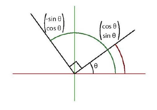
All Orthonormal Bases for \(\mathbb{R}^{2}\)

We wish to find all orthonormal bases for the space \(\mathbb{R}^{2}\), and they are \(\{ e_{1}^{\theta}, e_{2}^{\theta} \}\) up to reordering where

\[\begin{array}{cc}e_{1}^{\theta} = \begin{pmatrix} \cos \theta \\ \sin \theta \end{pmatrix}, & e_{2}^{\theta} = \begin{pmatrix} -\sin \theta \\ \cos \theta \end{pmatrix},\end{array}\]

for some \(\theta \in [0, 2\pi)\). Now first we need to show that for a fixed \(\theta\) that the pair is orthogonal:

\[e_{1}^{\theta} \cdot e_{2}^{\theta} = -\sin \theta \cos \theta + \cos \theta \sin \theta = 0.\]

Also we have

\[\norm{e_{1}^{\theta}}^{2} = \norm{e_{2}^{\theta}}^{2} = \sin^{2} \theta + \cos^{2} \theta = 1,\]

and hence \(\{ e_{1}^{\theta}, e_{2}^{\theta} \}\) is an orthonormal basis. To show that every orthonormal basis of \(\mathbb{R}^{2}\) is \(\{ e_{1}^{\theta}, e_{2}^{\theta} \}\) for some \(\theta\), consider an orthonormal basis \(\{ b_{1}, b_{2} \}\) and note that \(b_{1}\) forms an angle \(\phi\) with the vector \(e_{1}\) (which is \(e_{1}^{0}\)). Thus \(b_{1} = e_{1}^{\phi}\) and if \(b_{2} = e_{2}^{\phi}\), we are done, otherwise \(b_{2} = -e_{2}^{\phi}\) and it is the reflected version. However we can do the same thing except starting with \(b_{2}\) and get \(b_{2} = e_{1}^{\psi}\) and \(b_{1} = e_{2}^{\psi}\) since we have just interchanged two basis vectors which corresponds to a reflection which picks up a minus sign as in the determinant.

A \(4\times 4\) Gram-Schmidt Example

Lets do an example of how to "Gram-Schmidt" some vectors in \(\mathbb{R}^{4}\). Given the following vectors

\[v_{1} = \begin{pmatrix}o\\1 \\ 0\\ 0\end{pmatrix}, \, v_{2} = \begin{pmatrix}0\\1\\ 1\\ 0\end{pmatrix}, \, v_{3} = \begin{pmatrix}3\\0 \\ 1\\ 0\end{pmatrix}, \, \text{ and } v_{4} = \begin{pmatrix}1\\ 1\\ 0\\2\end{pmatrix},\]

we start with \(v_{1}\)

\[v_{1}^{\bot} = v_{1} =\begin{pmatrix}0\\1 \\ 0\\ 0\end{pmatrix}.\]

Now the work begins

\begin{eqnarray*}v_{2}^{\bot} &=& v_{2} -\frac{(v_{1}^{\bot} \cdot v_{2}) }{\norm{v_{1}^{\bot}}^{2}} v_{1}^{\bot} \\&=&\begin{pmatrix}0\\1\\ 1\\ 0\end{pmatrix} - \frac{1}{1} \begin{pmatrix}0\\1 \\ 0\\ 0\end{pmatrix}\\&=& \begin{pmatrix}0\\0\\ 1\\ 0\end{pmatrix} \\\end{eqnarray*}

This gets a little longer with every step.

\begin{eqnarray*}v_{3}^{\bot} &=& v_{3} -\frac{(v_{1}^{\bot} \cdot v_{3} )}{\norm{v_{1}^{\bot}}^{2}} v_{1}^{\bot} -\frac{(v_{2}^{\bot} \cdot v_{3} )}{\norm{v_{2}^{\bot}}^{2}} v_{2}^{\bot}\\&=&\begin{pmatrix}3\\0 \\ 1\\ 0\end{pmatrix}- \frac{0}{1} \begin{pmatrix}0\\1 \\ 0\\ 0\end{pmatrix} - \frac{1}{1} \begin{pmatrix}0\\0\\ 1\\ 0\end{pmatrix} = \begin{pmatrix}3\\0 \\ 0\\ 0\end{pmatrix}\\\end{eqnarray*}

This last step requires subtracting off the term of the form \(\frac{u\cdot v}{u \cdot u} \mathbf{u}\) for each of the previously defined basis vectors.

\begin{eqnarray*}v_{4}^{\bot} &=& v_{4} - \frac{(v_{1}^{\bot} \cdot v_{4} )}{\norm{v_{1}^{\bot}}^{2}} v_{1}^{\bot} -\frac{(v_{2}^{\bot} \cdot v_{4} )}{\norm{v_{2}^{\bot}}^{2}} v_{2}^{\bot} -\frac{(v_{3}^{\bot} \cdot v_{4} )}{\norm{v_{3}^{\bot}}^{2}} v_{3}^{\bot} \\&=& \begin{pmatrix}1\\ 1\\ 0\\2\end{pmatrix} -\frac{1}{1} \begin{pmatrix}0\\1 \\ 0\\ 0\end{pmatrix} - \frac{0}{1} \begin{pmatrix}0\\0\\ 1\\ 0\end{pmatrix} -\frac{3}{9} \begin{pmatrix}3\\0 \\ 0\\ 0\end{pmatrix} \\&=& \begin{pmatrix}0\\ 0\\ 0\\2\end{pmatrix}\end{eqnarray*}

Now \(v_{1}^{\bot}\), \(v_{2}^{\bot}\), \(v_{3}^{\bot}\), and \(v_{4}^{\bot}\) are an orthogonal basis. Notice that even with very, very nice looking vectors we end up having to do quite a bit of arithmetic. This a good reason to use programs like matlab to check your work.

Another \(QR\) Decomposition Example

We can alternatively think of the \(QR\) decomposition as performing the Gram-Schmidt procedure on the \(\textit{column space}\), the vector space of the column vectors of the matrix, of the matrix \(M\). The resulting orthonormal basis will be stored in \(Q\) and the negative of the coefficients will be recorded in \(R\). Note that \(R\) is upper triangular by how Gram-Schmidt works. Here we will explicitly do an example with the matrix

\[M = \begin{pmatrix} | & | & | \\m_{1} & m_{2} & m_{3} \\ | & | & | \end{pmatrix} = \begin{pmatrix}1 & 1 & -1 \\0 & 1 & 2 \\-1 & 1 & 1\end{pmatrix}.\]

First we normalize \(m_{1}\) to get \(m_{1}^{\prime} = \frac{m_{1}}{\norm{m_{1}}}\) where \(\norm{m_{1}} = r_{1}^{1} = \sqrt{2}\) which gives the decomposition

\[Q_{1} = \begin{pmatrix}\frac{1}{\sqrt{2}} & 1 & -1 \\0 & 1 & 2 \\-\frac{1}{\sqrt{2}} & 1 & 1\end{pmatrix},R_{1} = \begin{pmatrix}\sqrt{2} & 0 & 0 \\0 & 1 & 0 \\0 & 0 & 1\end{pmatrix}.\]

Next we find

\[t_{2} = m_{2} - (m_{1}^{\prime} \cdot m_{2}) m_{1}^{\prime} = m_{2} - r^{1}_{2} m^{\prime}_{1} = m_{2} - 0 m_{1}^{\prime}\]

noting that

\[m_{1}^{\prime} \cdot m_{1}^{\prime} = \norm{m_{1}^{\prime}}^{2} = 1\]

and \(\norm{t_{2}} = r^{2}_{2} = \sqrt{3}\), and so we get \(m_{2}^{\prime} = \frac{t_{2}}{\norm{t_{2}}}\) with the decomposition

\[Q_{2} = \begin{pmatrix}\frac{1}{\sqrt{2}} & \frac{1}{\sqrt{3}} & -1 \\0 & \frac{1}{\sqrt{3}} & 2 \\-\frac{1}{\sqrt{2}} & \frac{1}{\sqrt{3}} & 1\end{pmatrix},R_{2} = \begin{pmatrix}\sqrt{2} & 0 & 0\\0 & \sqrt{3} & 0 \\0 & 0 & 1\end{pmatrix}.\]

Finally we calculate

\begin{align*}t_{3} & = m_{3} - (m_{1}^{\prime} \cdot m_{3}) m_{1}^{\prime} - (m_{2}^{\prime} \cdot m_{3}) m_{2}^{\prime}\\ & = m_{3} - r^{1}_{3} m_{1}^{\prime} - r^{2}_{3} m_{2}^{\prime} = m_{3} + \sqrt{2} m_{1}^{\prime} - \frac{2}{\sqrt{3}} m_{2}^{\prime},\end{align*}

again noting \(m_{2}^{\prime} \cdot m_{2}^{\prime} = \norm{m_{2}^{\prime}} = 1\), and let \(m_{3}^{\prime} = \frac{t_{3}}{\norm{t_{3}}}\) where \(\norm{t_{3}} = r^{3}_{3} = 2 \sqrt{\frac{2}{3}}\). Thus we get our final \(M = QR\) decomposition as

\[Q = \begin{pmatrix}\frac{1}{\sqrt{2}} & \frac{1}{\sqrt{3}} & - \frac{1}{\sqrt{2}} \\0 & \frac{1}{\sqrt{3}} & \sqrt{\frac{2}{3}} \\-\frac{1}{\sqrt{2}} & \frac{1}{3} & - \frac{1}{\sqrt{6}}\end{pmatrix},R = \begin{pmatrix}\sqrt{2} & 0 & -\sqrt{2} \\0 & \sqrt{3} & \frac{2}{\sqrt{3}} \\0 & 0 & 2 \sqrt{\frac{2}{3}}\end{pmatrix}.\]

Overview

This video considers solutions sets for linear systems with three unknowns. These are often called \((x,y,z)\) and label points in \(\mathbb{R}^{3}\). Lets work case by case:

1. If you have no equations at all, then any \((x,y,z)\) is a solution, so the solution set is all of \(\mathbb{R}^{3}\). The picture looks a little silly: (Fig1)
2. For a single equation, the solution is a plane. The picture looks like this:​ (Fig2)
3. For two equations, we must look at two planes. These usually intersect along a line, so the solution set will also (usually) be a line: (Fig3)
4. For three equations, most often their intersection will be a single point so the solution will then be unique: (Fig4)
5. Of course stuff can go wrong. Two different looking equations could determine the same plane, or worse equations could be inconsistent. If the equations are inconsistent, there will be no solutions at all. For example, if you had four equations determining four parallel planes the solution set would be empty. This looks like this: (Fig5)

​

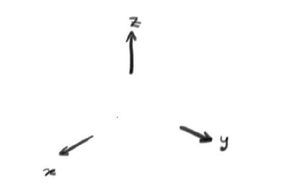
Fig1: \(R^{3}\)

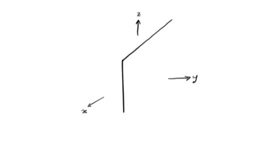
Fig2: Plane in \(R^{3}\)

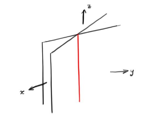
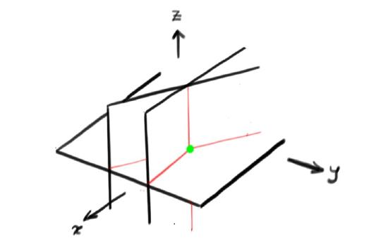
Fig3: Two Planes in \(R^{3}\) Fig4: Three Planes in \(R^{3}\)

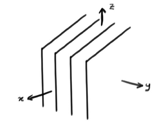
Fig5: Four Planes in \(R^{3}\)

Hint for Review Question 2

You are asked to consider an orthogonal basis \(\{v_{1},v_{2},\ldots v_{n}\}\). Because this is a basis any \(v\in V\) can be uniquely expressed as

$$v=c^{1} v_{1} + c^{2} v_{2} +\cdots + v^{n} c_{n}\, ,\]

and the number \(n=\dim V\). Since this is an orthogonal basis

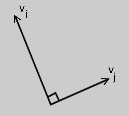
$$v_{i}\cdot v_{j} =0 \, ,\qquad i\neq j\, .\]

So different vectors in the basis are orthogonal:

However, the basis is \(\textit{not}\) orthonormal so we know nothing about the lengths of the basis vectors (save that they cannot vanish).

To complete the hint, lets use the dot product to compute a formula for \(c^{1}\) in terms of the basis vectors and \(v\). Consider

$$v_{1}\cdot v = c^{1} v_{1}\cdot v_{1} + c^{2} v_{1}\cdot v^{2} +\cdots + c^{n} v_{1}\cdot v_{n}=c^{1} v_{1}\cdot v_{1}\, .\]

Solving for \(c^{1}\) (remembering that \(v_{1}\cdot v_{1}\neq 0\)) gives

\[c^{1} = \frac{v_{1}\cdot v}{v_{1}\cdot v_{1}}\, .\]

This should get you started on this problem.

Hint for Review Problem 3

Lets work part by part:

1. Is the vector \(v^(\bot) = v-\frac{u\cdot v}{u\cdot u}u\) in the plane \(P\)? Remember that the dot product gives you a scalar not a vector, so if you think about this formula \(\frac{\mathbf{u}\cdot \mathbf{v}}{\mathbf{u}\cdot \mathbf{u}}\) is a scalar, so this is a linear combination of \(\mathbf{v}\) and \(\mathbf{u}\). Do you think it is in the span?
2. What is the angle between \(v^{\bot}\) and \(u\)? This part will make more sense if you think back to the dot product formulas you probably first saw in multivariable calculus. Remember that \[\mathbf{u}\cdot \mathbf{v} = \norm{\mathbf{u}} \norm{\mathbf{v}} \cos(\theta),\] and in particular if they are perpendicular \(\theta = \frac{\pi}{2}\) and \(\cos(\frac{\pi}{2}) = 0\) you will get \(\mathbf{u}\cdot \mathbf{v} = 0\). Now try to compute the dot product of \(u\) and \(v^{\bot}\) to find \(\norm{\mathbf{u}} \norm{\mathbf{v^{\bot}}} \cos(\theta)\) \begin{eqnarray*}u\cdot v^{\bot} &=& u\cdot \left( v - \frac{u\cdot v}{u\cdot u}u \right) \\&=& u\cdot v - u\cdot \left( \frac{u\cdot v}{u\cdot u} \right)u \\&=& u\cdot v - \left( \frac{u\cdot v}{u\cdot u} \right) u\cdot u \\\end{eqnarray*} Now you finish simplifying and see if you can figure out what \(\theta\) has to be.
3. Given your solution to the above, how can you find a third vector perpendicular to both \(u\) and \(v^{\bot}\)? Remember what other things you learned in multivariable calculus? This might be a good time to remind your self what the cross product does.
4. Construct an orthonormal basis for \(\Re^{3}\) from \(u\) and \(v\). If you did part (c) you can probably find 3 orthogonal vectors to make a orthogonal basis. All you need to do to turn this into an orthonormal basis is make these into unit vectors.
5. Test your abstract formulae starting with \[u=\begin{pmatrix}1 & 2 & 0\end{pmatrix} \text{ and } v=\begin{pmatrix}0 & 1 & 1\end{pmatrix}.\] Try it out, and if you get stuck try drawing a sketch of the vectors you have.

Hint for Review Problem 10

This video shows you a way to solve problem 10 that's different to the method described in the lecture. The first thing is to think of $$M = \begin{pmatrix}1 & 0 & 2 \\ -1 & 2 & 0 \\ -1 & 2 & 2\end{pmatrix}$$ as a set of 3 vectors $$v_{1}=\begin{pmatrix}0\\-1\\-1\end{pmatrix}, v_{2}=\begin{pmatrix}0\\2\\-2\end{pmatrix}, v_{3}=\begin{pmatrix}2\\0\\2\end{pmatrix}.$$ Then you need to remember that we are searching for a decomposition $$M = QR\]

where \(Q\) is an orthogonal matrix. Thus the upper triangular matrix \(R = Q^{T}M\) and \(Q^{T}Q = I\). Moreover, orthogonal matrices perform rotations. To see this, compare the inner product \(u\cdot v = u^{T} v\) of vectors \(u\) and \(v\) with that of \(Qu\) and \(Qv\):

\[(Qu)\cdot (Qv) = (Qu)^{T}(Qv) = u^{T}Q^{T}Qv = u^{T}v = u\cdot v.\]

Since the dot product doesn't change, we learn that \(Q\) does not change angles or lengths of vectors. Now, here's an interesting procedure: rotate \(v_{1}, v_{2}\) and \(v_{3}\) such that \(v_{1}\) is along the x-axis, \(v_{2}\) is in the xy-plane. Then if you put these in a matrix you get something of the form

\[\begin{pmatrix}a & b & c \\ 0 & d & e \\ 0 & 0 & f\end{pmatrix}\]

which is exactly what we don't want for \(R!\)

Moreover, the vector

\[\begin{pmatrix}a\\0\\0\end{pmatrix}\]

is the rotated \(v_{1}\) so must have length \(||v_{1}|| = \sqrt{3}\). Thus \(a = \sqrt{3}\). The rotated \(v_{2}\) is

\[\begin{pmatrix}b\\d\\0\end{pmatrix}\]

and must have length \(||v_{2}|| = 2\sqrt{2}\). Also the dot product between

\[\begin{pmatrix}a\\0\\0\end{pmatrix} \text{ and } \begin{pmatrix}b\\d\\0\end{pmatrix}\]

is \(ab\) and must equal \(v_{1}\cdot v_{2} = 0\). (That \(v_{1}\) and \(v_{2}\) were orthogonal is just a coincidence here….). Thus \(b=0\). So now we know most of the matrix \(R\)

\[R=\begin{pmatrix}\sqrt{3} & 0 & c \\ 0 & 2\sqrt{2} & e \\ 0 & 0 & f\end{pmatrix}\]

You can work out the last column using the same ideas. Thus it only remains to compute \(Q\) from

\[Q = MR^{-1}.\]

G.14 Diagonalizing Symmetric Matrices

\(3 \times 3\) Example

Lets diagonalize the matrix

\[M =\begin{pmatrix}1 &2 & 0 \\2 & 1 & 0 \\0& 0 & 5 \\\end{pmatrix}\]

If we want to diagonalize this matrix, we should be happy to see that it is symmetric, since this means we will have real eigenvalues, which means factoring won't be too hard. As an added bonus if we have three distinct eigenvalues the eigenvectors we find will automatically be orthogonal, which means that the inverse of the matrix \(P\) will be easy to compute. We can start by finding the eigenvalues of this

\begin{eqnarray*}\det \begin{pmatrix}1-\lambda & 2 & 0 \\2 & 1 -\lambda& 0 \\0& 0 & 5-\lambda \\\end{pmatrix}&=& (1-\lambda)\begin{vmatrix}1 -\lambda& 0 \\0 & 5-\lambda \\\end{vmatrix}\\ & & - \, (2)\begin{vmatrix}2 & 0 \\0& 5-\lambda \\\end{vmatrix}+ 0 \begin{vmatrix}2 & 1 -\lambda \\0& 0 \\\end{vmatrix}\\&=&(1-\lambda)(1-\lambda)(5-\lambda)+ (-2)(2)(5-\lambda) +0\\&=&(1-2\lambda +\lambda^{2})(5-\lambda) + (-2)(2)(5-\lambda)\\&=&((1-4 )-2\lambda +\lambda^{2})(5-\lambda)\\&=&(-3-2\lambda +\lambda^{2})(5-\lambda)\\&=&(1+\lambda)(3-\lambda)(5-\lambda)\\\end{eqnarray*}

So we get \(\lambda = -1, 3, 5\) as eigenvectors. First find \(v_{1}\) for \(\lambda_{1} = -1\)

\[(M+I)\begin{pmatrix}x\\y\\z\end{pmatrix}=\begin{pmatrix}2 &2 & 0 \\2 & 2& 0 \\0& 0 & 6 \\\end{pmatrix}\begin{pmatrix}x\\y\\z\end{pmatrix}= \begin{pmatrix}0\\0\\0\end{pmatrix},\]

implies that \(2x+2y= 0\) and \(6z = 0\), which means any multiple of \(v_{1} = \begin{pmatrix}1\\-1\\0\end{pmatrix}\) is an eigenvector with eigenvalue \(\lambda_{1} = -1\). Now for \(v_{2}\) with \(\lambda_{2} = 3\)

\[(M-3I)\begin{pmatrix}x\\y\\z\end{pmatrix}=\begin{pmatrix}-2 &2 & 0 \\2 & -2& 0 \\0& 0 & 4 \\\end{pmatrix}\begin{pmatrix}x\\y\\z\end{pmatrix}= \begin{pmatrix}0\\0\\0\end{pmatrix},\]

and we can find that that \(v_{2} = \begin{pmatrix}1\\1\\0\end{pmatrix} would satisfy \(-2x+2y= 0\), \(2x-2y= 0\) and \(4z = 0\).

Now for \(v_{3}\) with \(\lambda_{3} = 5\)

\[(M-5I)\begin{pmatrix}x\\y\\z\end{pmatrix}=\begin{pmatrix}-4 &2 & 0 \\2 & -4& 0 \\0& 0 & 0 \\\end{pmatrix}\begin{pmatrix}x\\y\\z\end{pmatrix}= \begin{pmatrix}0\\0\\0\end{pmatrix},\]

Now we want \(v_{3}\) to satisfy \(-4 x+ 2y = 0\) and \(2 x-4 y = 0\), which imply \(x=y=0\), but since there are no restrictions on the \(z\) coordinate we have \(v_{3} = \begin{pmatrix}0\\0\\1\end{pmatrix}\).

Notice that the eigenvectors form an orthogonal basis. We can create an orthonormal basis by rescaling to make them unit vectors. This will help us because if \(P = [v_{1},v_{2},v_{3}]\) is created from orthonormal vectors then \(P^{-1}=P^{T}\), which means computing \(P^{-1}\) should be easy. So lets say

\[v_{1} = \begin{pmatrix}\frac{1}{\sqrt{2}}\\-\frac{1}{\sqrt{2}}\\0\end{pmatrix}, \, v_{2} = \begin{pmatrix}\frac{1}{\sqrt{2}}\\\frac{1}{\sqrt{2}}\\0\end{pmatrix}, \text{ and } v_{3} = \begin{pmatrix}0\\0\\1\end{pmatrix}\]

so we get

\[P=\begin{pmatrix}\frac{1}{\sqrt{2}} & \frac{1}{\sqrt{2}}& 0\\-\frac{1}{\sqrt{2}} &\frac{1}{\sqrt{2}}& 0\\0&0 & 1\end{pmatrix} \text{ and }P^{-1}=\begin{pmatrix}\frac{1}{\sqrt{2}} & -\frac{1}{\sqrt{2}}& 0\\\frac{1}{\sqrt{2}} &\frac{1}{\sqrt{2}}& 0\\0&0 & 1\end{pmatrix}\]

So when we compute \(D= P^{-1} M P\) we'll get

\[\begin{pmatrix}\frac{1}{\sqrt{2}} & -\frac{1}{\sqrt{2}}& 0\\\frac{1}{\sqrt{2}} &\frac{1}{\sqrt{2}}& 0\\0&0 & 1\end{pmatrix}\begin{pmatrix}1 &2 & 0 \\2 & 5 & 0 \\0& 0 & 5 \\\end{pmatrix}\begin{pmatrix}\frac{1}{\sqrt{2}} & \frac{1}{\sqrt{2}}& 0\\-\frac{1}{\sqrt{2}} &\frac{1}{\sqrt{2}}& 0\\0&0 & 1\end{pmatrix}= \begin{pmatrix}-1 &0 & 0 \\0 & 3 & 0 \\0& 0 & 5 \\\end{pmatrix}\]

Hint for Review Problem 1

For part (a), we can consider} any complex number \(z\) as being a vector in \(\mathbb{R}^{2}\) where complex conjugation corresponds to the matrix \(\begin{pmatrix} 1 & 0 \\ 0 & -1 \end{pmatrix}\). Can you describe \(z \bar{z}\) in terms of \(\norm{z}\)? For part (b), think about what values \(a \in \mathbb{R}\) can take if \(a = -a\)? Part (c), just compute it and look back at part (a).

For part (d), note that \(x^{\dagger} x\) is just a number, so we can divide by it. Parts (e) and (f) follow right from definitions. For part (g), first notice that every row vector is the (unique) transpose of a column vector, and also think about why \((A A^{T})^{T} = A A^{T}\) for any matrix \(A\). Additionally you should see that \(\overline{x^{T}} = x^{\dagger}\) and mention this. Finally for part (h), show that

\[\frac{x^{\dagger} M x}{x^{\dagger} x} = \overline{\left(\frac{x^{\dagger} M x}{x^{\dagger} x}\right)^{T}}\]

and reduce each side separately to get \(\lambda = \overline{\lambda}\).

Contributor

• David Cherney, Tom Denton, and Andrew Waldron (UC Davis)