8.2: The Cartesian Coordinate System
- Page ID
- 22509
\( \newcommand{\vecs}[1]{\overset { \scriptstyle \rightharpoonup} {\mathbf{#1}} } \)
\( \newcommand{\vecd}[1]{\overset{-\!-\!\rightharpoonup}{\vphantom{a}\smash {#1}}} \)
\( \newcommand{\dsum}{\displaystyle\sum\limits} \)
\( \newcommand{\dint}{\displaystyle\int\limits} \)
\( \newcommand{\dlim}{\displaystyle\lim\limits} \)
\( \newcommand{\id}{\mathrm{id}}\) \( \newcommand{\Span}{\mathrm{span}}\)
( \newcommand{\kernel}{\mathrm{null}\,}\) \( \newcommand{\range}{\mathrm{range}\,}\)
\( \newcommand{\RealPart}{\mathrm{Re}}\) \( \newcommand{\ImaginaryPart}{\mathrm{Im}}\)
\( \newcommand{\Argument}{\mathrm{Arg}}\) \( \newcommand{\norm}[1]{\| #1 \|}\)
\( \newcommand{\inner}[2]{\langle #1, #2 \rangle}\)
\( \newcommand{\Span}{\mathrm{span}}\)
\( \newcommand{\id}{\mathrm{id}}\)
\( \newcommand{\Span}{\mathrm{span}}\)
\( \newcommand{\kernel}{\mathrm{null}\,}\)
\( \newcommand{\range}{\mathrm{range}\,}\)
\( \newcommand{\RealPart}{\mathrm{Re}}\)
\( \newcommand{\ImaginaryPart}{\mathrm{Im}}\)
\( \newcommand{\Argument}{\mathrm{Arg}}\)
\( \newcommand{\norm}[1]{\| #1 \|}\)
\( \newcommand{\inner}[2]{\langle #1, #2 \rangle}\)
\( \newcommand{\Span}{\mathrm{span}}\) \( \newcommand{\AA}{\unicode[.8,0]{x212B}}\)
\( \newcommand{\vectorA}[1]{\vec{#1}} % arrow\)
\( \newcommand{\vectorAt}[1]{\vec{\text{#1}}} % arrow\)
\( \newcommand{\vectorB}[1]{\overset { \scriptstyle \rightharpoonup} {\mathbf{#1}} } \)
\( \newcommand{\vectorC}[1]{\textbf{#1}} \)
\( \newcommand{\vectorD}[1]{\overrightarrow{#1}} \)
\( \newcommand{\vectorDt}[1]{\overrightarrow{\text{#1}}} \)
\( \newcommand{\vectE}[1]{\overset{-\!-\!\rightharpoonup}{\vphantom{a}\smash{\mathbf {#1}}}} \)
\( \newcommand{\vecs}[1]{\overset { \scriptstyle \rightharpoonup} {\mathbf{#1}} } \)
\(\newcommand{\longvect}{\overrightarrow}\)
\( \newcommand{\vecd}[1]{\overset{-\!-\!\rightharpoonup}{\vphantom{a}\smash {#1}}} \)
\(\newcommand{\avec}{\mathbf a}\) \(\newcommand{\bvec}{\mathbf b}\) \(\newcommand{\cvec}{\mathbf c}\) \(\newcommand{\dvec}{\mathbf d}\) \(\newcommand{\dtil}{\widetilde{\mathbf d}}\) \(\newcommand{\evec}{\mathbf e}\) \(\newcommand{\fvec}{\mathbf f}\) \(\newcommand{\nvec}{\mathbf n}\) \(\newcommand{\pvec}{\mathbf p}\) \(\newcommand{\qvec}{\mathbf q}\) \(\newcommand{\svec}{\mathbf s}\) \(\newcommand{\tvec}{\mathbf t}\) \(\newcommand{\uvec}{\mathbf u}\) \(\newcommand{\vvec}{\mathbf v}\) \(\newcommand{\wvec}{\mathbf w}\) \(\newcommand{\xvec}{\mathbf x}\) \(\newcommand{\yvec}{\mathbf y}\) \(\newcommand{\zvec}{\mathbf z}\) \(\newcommand{\rvec}{\mathbf r}\) \(\newcommand{\mvec}{\mathbf m}\) \(\newcommand{\zerovec}{\mathbf 0}\) \(\newcommand{\onevec}{\mathbf 1}\) \(\newcommand{\real}{\mathbb R}\) \(\newcommand{\twovec}[2]{\left[\begin{array}{r}#1 \\ #2 \end{array}\right]}\) \(\newcommand{\ctwovec}[2]{\left[\begin{array}{c}#1 \\ #2 \end{array}\right]}\) \(\newcommand{\threevec}[3]{\left[\begin{array}{r}#1 \\ #2 \\ #3 \end{array}\right]}\) \(\newcommand{\cthreevec}[3]{\left[\begin{array}{c}#1 \\ #2 \\ #3 \end{array}\right]}\) \(\newcommand{\fourvec}[4]{\left[\begin{array}{r}#1 \\ #2 \\ #3 \\ #4 \end{array}\right]}\) \(\newcommand{\cfourvec}[4]{\left[\begin{array}{c}#1 \\ #2 \\ #3 \\ #4 \end{array}\right]}\) \(\newcommand{\fivevec}[5]{\left[\begin{array}{r}#1 \\ #2 \\ #3 \\ #4 \\ #5 \\ \end{array}\right]}\) \(\newcommand{\cfivevec}[5]{\left[\begin{array}{c}#1 \\ #2 \\ #3 \\ #4 \\ #5 \\ \end{array}\right]}\) \(\newcommand{\mattwo}[4]{\left[\begin{array}{rr}#1 \amp #2 \\ #3 \amp #4 \\ \end{array}\right]}\) \(\newcommand{\laspan}[1]{\text{Span}\{#1\}}\) \(\newcommand{\bcal}{\cal B}\) \(\newcommand{\ccal}{\cal C}\) \(\newcommand{\scal}{\cal S}\) \(\newcommand{\wcal}{\cal W}\) \(\newcommand{\ecal}{\cal E}\) \(\newcommand{\coords}[2]{\left\{#1\right\}_{#2}}\) \(\newcommand{\gray}[1]{\color{gray}{#1}}\) \(\newcommand{\lgray}[1]{\color{lightgray}{#1}}\) \(\newcommand{\rank}{\operatorname{rank}}\) \(\newcommand{\row}{\text{Row}}\) \(\newcommand{\col}{\text{Col}}\) \(\renewcommand{\row}{\text{Row}}\) \(\newcommand{\nul}{\text{Nul}}\) \(\newcommand{\var}{\text{Var}}\) \(\newcommand{\corr}{\text{corr}}\) \(\newcommand{\len}[1]{\left|#1\right|}\) \(\newcommand{\bbar}{\overline{\bvec}}\) \(\newcommand{\bhat}{\widehat{\bvec}}\) \(\newcommand{\bperp}{\bvec^\perp}\) \(\newcommand{\xhat}{\widehat{\xvec}}\) \(\newcommand{\vhat}{\widehat{\vvec}}\) \(\newcommand{\uhat}{\widehat{\uvec}}\) \(\newcommand{\what}{\widehat{\wvec}}\) \(\newcommand{\Sighat}{\widehat{\Sigma}}\) \(\newcommand{\lt}{<}\) \(\newcommand{\gt}{>}\) \(\newcommand{\amp}{&}\) \(\definecolor{fillinmathshade}{gray}{0.9}\)Let’s begin with the concept of an ordered pair of whole numbers.
The construct (x, y), where x and y are whole numbers, is called an ordered pair of whole numbers.
Examples of ordered pairs of whole numbers are (0, 0), (2, 3), (5, 1), and (4, 9).
Pay particular attention to the phrase “ordered pairs.” Order matters. Consequently, the ordered pair (x, y) is not the same as the ordered pair (y, x), because the numbers are presented in a different order.
We’ve seen how to plot whole numbers on a number line. For example, in Figure 8.1, we’ve plotted the whole numbers 2, 5, and 7 as shaded “dots” on the number line.

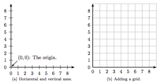
To plot ordered pairs, we need two number lines, called the horizontal and vertical axes, that intersect at the zero location of each line and are at right angles to one another, as shown in Figure 8.2(a). The point where the zero locations touch is called the origin of the coordinate system and has coordinates (0, 0). In Figure 8.2(b), we’ve added a grid. The resulting construct is an example of a Cartesian Coordinate System.
Now, consider the ordered pair of whole numbers (5, 6). To plot this point on the “coordinate system” in Figure 8.3(a), start at the origin (0, 0), then move 5 units in the horizontal direction, then 6 units in the vertical direction, then plot a point. The result is shown in Figure 8.3(a). Adding a grid of horizontal and vertical lines at each whole number makes plotting the point (5, 6) much clearer, as shown in Figure 8.3(b).
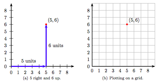
The numbers in the ordered pair (5, 6) are called the coordinates of the plotted point in Figure 8.3(b). The first number of the ordered pair is called the abscissa and measures the horizontal distance to the plotted point. The second number is called the ordinate and measures the vertical distance to the plotted point. The combination of axes and grid in Figure 8.3(b) is called a coordinate system.
The grid in Figure 8.3(b) is a visualization that greatly eases the plotting of ordered pairs. However, you do not have to draw these gridlines yourself. Instead, you should work on graph paper.
All plotting should be done on graph paper.
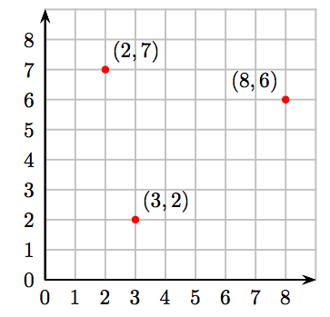
Plot the following ordered pairs of whole numbers: (3, 2), (8, 6), and (2, 7).
Solution
Create a Cartesian coordinate system on graph paper, then:
- To plot the ordered pair (3, 2), start at the origin, then move 3 units to the right and 2 units up.
- To plot the ordered pair (8, 6), start at the origin, then move 8 units to the right and 6 units up.
- To plot the ordered pair (2, 7), start at the origin, then move 2 units to the right and 7 units up.
The results are shown on the following Cartesian coordinate system.
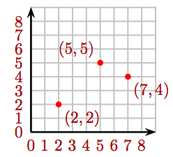
Plot the following ordered pairs of whole numbers: (2, 2), (5, 5), and (7, 4).
- Answer
-
Allowing for Negative Numbers
Again, we’ve seen how to plot both positive and negative numbers on a number line. For example, in Figure 8.4, we’ve plotted the numbers −4, −3/2, 2.2 and 4.

Note that the positive direction is to the right, the negative to the left. That is, to plot the number 2.2, we move 2.2 units to the right on the line, but to plot the number −3/2, we move 3/2 units to the left.
To plot ordered pairs having both positive and negative numbers, we need two such number lines that intersect at the zero location of each line and are at right angles to one another, as shown in Figure 8.5(a). As before, adding a grid of horizontal and vertical lines at each integer will be extremely helpful when plotting points (see Figure 8.5(b)). The system of axes and grid in Figure 8.5(b) is called the Cartesian Coordinate System, named after its inventor, René Descartes.
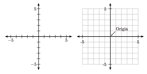
On the horizontal axis, the positive direction is to the right, negative is to the left. On the vertical axis, the positive direction is up, negative is down. The point (0, 0) is called the origin of the coordinate system, and is the starting point for all point plotting.
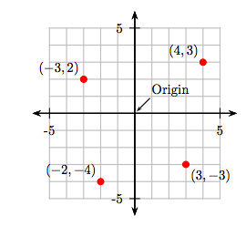
Sketch the points (4, 3), (−3, 2), (−2, −4), and (3, −3) on a Cartesian coordinate system.
Solution
Set up a Cartesian coordinate system on graph paper.
- To plot the point (4, 3), start at the origin, move 4 units to the right, then 3 units up.
- To plot the point (−3, 2), start at the origin, move 3 units to the left, then 2 units up.
- To plot the point (−2, −4), start at the origin, move 2 units to the left, then 4 units down.
- To plot the point (3, −3), start at the origin, move 3 units to the right, then 3 units down.
These points are plotted and shown in Figure 8.6.
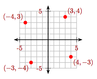
Sketch the points (3, 4), (−4, 3), (−3, −4), and (4, −3) on a Cartesian coordinate system.
- Answer
-
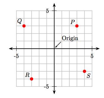
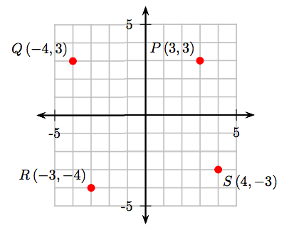
What are the coordinates of the points P, Q, R, and S in the Cartesian coordinate system that follows?
Solution
Make all measurements from the origin.
- To obtain the coordinates of point P, start at the origin, move 3 units to the right, then 3 units up. Hence, the coordinates of the point P are (3, 3).
- To obtain the coordinates of point Q, start at the origin, move 4 units to the left, then 3 units up. Hence, the coordinates of the point Q are (−4, 3).
- To obtain the coordinates of point R, start at the origin, move 3 units to the left, then 4 units down. Hence, the coordinates of the point R are (−3, −4).
- To obtain the coordinates of point S, start at the origin, move 4 units to the right, then 3 units down. Hence, the coordinates of the point S are (4, −3).
These results are shown on the following Cartesian coordinate system.
Exercises
1. Identify the coordinates of the point P.
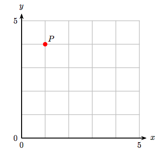
2. Identify the coordinates of the point P.
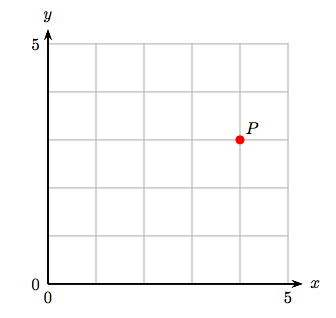
3. Identify the coordinates of the point P.
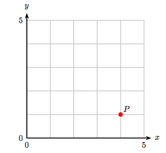
4. Identify the coordinates of the point P.
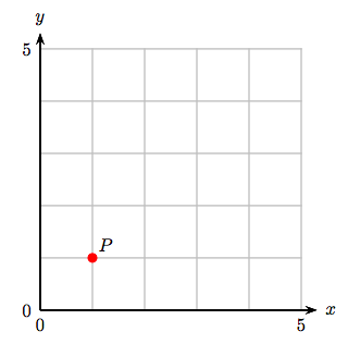
5. Identify the coordinates of the point P.
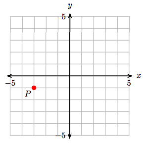
6. Identify the coordinates of the point P.
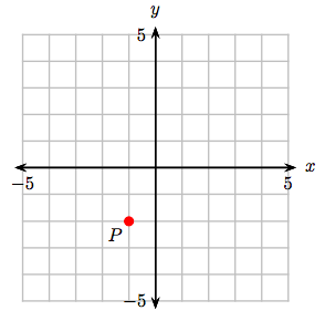
7. Identify the coordinates of the point P.
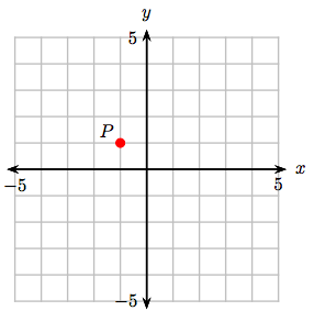
8. Identify the coordinates of the point P.
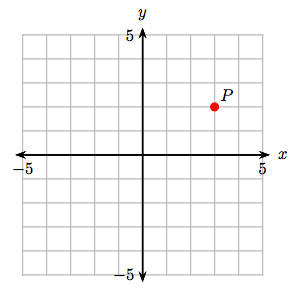
9. The points A(−1, 1), B(1, 1), C(1, 2), and D(−1, 2) are the vertices of a rectangle. Plot these points, draw the rectangle ABCD, then compute the area of rectangle ABCD.
10. The points A(−3, −4), B(4, −4), C(4, −1), and D(−3, −1) are the vertices of a rectangle. Plot these points, draw the rectangle ABCD, then compute the area of rectangle ABCD.
11. The points A(−2, −1), B(3, −1), C(3, 3), and D(−2, 3) are the vertices of a rectangle. Plot these points, draw the rectangle ABCD, then compute the area of rectangle ABCD.
12. The points A(−3, −1), B(2, −1), C(2, 2), and D(−3, 2) are the vertices of a rectangle. Plot these points, draw the rectangle ABCD, then compute the area of rectangle ABCD.
13. The points A(−4, −2), B(1, −2), C(1, 1), and D(−4, 1) are the vertices of a rectangle. Plot these points, draw the rectangle ABCD, then compute the perimeter of rectangle ABCD.
14. The points A(−4, −4), B(1, −4), C(1, −3), and D(−4, −3) are the vertices of a rectangle. Plot these points, draw the rectangle ABCD, then compute the perimeter of rectangle ABCD.
15. The points A(−1, 2), B(3, 2), C(3, 3), and D(−1, 3) are the vertices of a rectangle. Plot these points, draw the rectangle ABCD, then compute the perimeter of rectangle ABCD.
16. The points A(−4, 2), B(3, 2), C(3, 4), and D(−4, 4) are the vertices of a rectangle. Plot these points, draw the rectangle ABCD, then compute the perimeter of rectangle ABCD.
17. The points A(−3, −1), B(1, −1), and C(−3, 0) are the vertices of a triangle. Plot these points, draw the triangle ABC, then compute the area of the triangle ABC.
18. The points A(−3, −2), B(1, −2), and C(−3, 2) are the vertices of a triangle. Plot these points, draw the triangle ABC, then compute the area of the triangle ABC.
19. The points A(−1, −2), B(0, −2), and C(−1, 0) are the vertices of a triangle. Plot these points, draw the triangle ABC, then compute the area of the triangle ABC.
20. The points A(−2, −3), B(−1, −3), and C(−2, 1) are the vertices of a triangle. Plot these points, draw the triangle ABC, then compute the area of the triangle ABC.
21. Plot the points A(−3, −3) and B(0, 0) and find the straight-line distance between the two points. Hint: Create a right triangle, then use the Pythagorean Theorem.
22. Plot the points A(−2, −3) and B(1, 2) and find the straight-line distance between the two points. Hint: Create a right triangle, then use the Pythagorean Theorem.
23. Plot the points A(−2, −3) and B(0, 0) and find the straight-line distance between the two points. Hint: Create a right triangle, then use the Pythagorean Theorem.
24. Plot the points A(−3, −2) and B(2, 2) and find the straight-line distance between the two points. Hint: Create a right triangle, then use the Pythagorean Theorem.
25. Find the area of the shaded triangle.
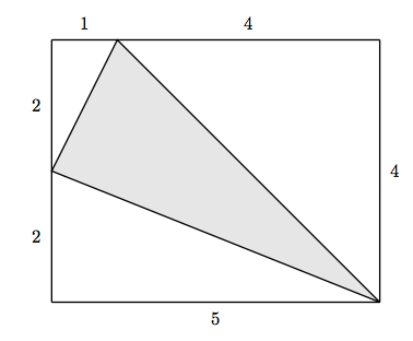
26. Find the area of the shaded triangle.
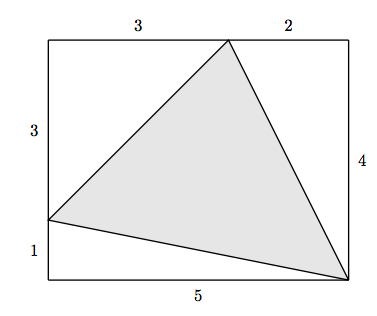
27. Find the area of the shaded triangle.
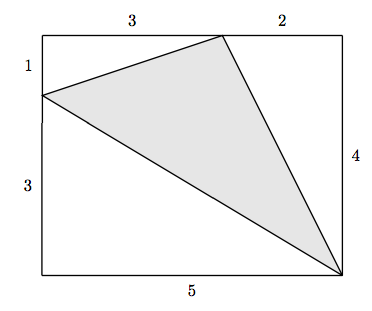
28. Find the area of the shaded triangle.
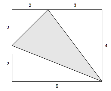
Hint: In Exercises 29-32, surround the triangle with a rectangle, like those shown in Exercises 25-28.
29. Find the area of the triangle with vertices at A(−4, −1), B(4, −2), and C(1, 3).
30. Find the area of the triangle with vertices at A(−4, 2), B(3, 0), and C(0, 4).
31. Find the area of the triangle with vertices at A(−3, 1), B(3, −3), and C(1, 4).
32. Find the area of the triangle with vertices at A(1, 2), B(3, 0), and C(2, 4).
Answers
1. (1, 4)
3. (4, 1)
5. (−3, −1)
7. (−1, 1)
9. 2 square units
11. 20 square units
13. 16 units
15. 10 units
17. 2 square units
19. 1 square units
21. \(\sqrt{18}\)
23. \(\sqrt{13}\)
25. 6
27. 7
29. \(\frac{37}{2}\)
31. 17


