11.E: Graphs (Exercises)
- Page ID
- 7296
\( \newcommand{\vecs}[1]{\overset { \scriptstyle \rightharpoonup} {\mathbf{#1}} } \)
\( \newcommand{\vecd}[1]{\overset{-\!-\!\rightharpoonup}{\vphantom{a}\smash {#1}}} \)
\( \newcommand{\dsum}{\displaystyle\sum\limits} \)
\( \newcommand{\dint}{\displaystyle\int\limits} \)
\( \newcommand{\dlim}{\displaystyle\lim\limits} \)
\( \newcommand{\id}{\mathrm{id}}\) \( \newcommand{\Span}{\mathrm{span}}\)
( \newcommand{\kernel}{\mathrm{null}\,}\) \( \newcommand{\range}{\mathrm{range}\,}\)
\( \newcommand{\RealPart}{\mathrm{Re}}\) \( \newcommand{\ImaginaryPart}{\mathrm{Im}}\)
\( \newcommand{\Argument}{\mathrm{Arg}}\) \( \newcommand{\norm}[1]{\| #1 \|}\)
\( \newcommand{\inner}[2]{\langle #1, #2 \rangle}\)
\( \newcommand{\Span}{\mathrm{span}}\)
\( \newcommand{\id}{\mathrm{id}}\)
\( \newcommand{\Span}{\mathrm{span}}\)
\( \newcommand{\kernel}{\mathrm{null}\,}\)
\( \newcommand{\range}{\mathrm{range}\,}\)
\( \newcommand{\RealPart}{\mathrm{Re}}\)
\( \newcommand{\ImaginaryPart}{\mathrm{Im}}\)
\( \newcommand{\Argument}{\mathrm{Arg}}\)
\( \newcommand{\norm}[1]{\| #1 \|}\)
\( \newcommand{\inner}[2]{\langle #1, #2 \rangle}\)
\( \newcommand{\Span}{\mathrm{span}}\) \( \newcommand{\AA}{\unicode[.8,0]{x212B}}\)
\( \newcommand{\vectorA}[1]{\vec{#1}} % arrow\)
\( \newcommand{\vectorAt}[1]{\vec{\text{#1}}} % arrow\)
\( \newcommand{\vectorB}[1]{\overset { \scriptstyle \rightharpoonup} {\mathbf{#1}} } \)
\( \newcommand{\vectorC}[1]{\textbf{#1}} \)
\( \newcommand{\vectorD}[1]{\overrightarrow{#1}} \)
\( \newcommand{\vectorDt}[1]{\overrightarrow{\text{#1}}} \)
\( \newcommand{\vectE}[1]{\overset{-\!-\!\rightharpoonup}{\vphantom{a}\smash{\mathbf {#1}}}} \)
\( \newcommand{\vecs}[1]{\overset { \scriptstyle \rightharpoonup} {\mathbf{#1}} } \)
\(\newcommand{\longvect}{\overrightarrow}\)
\( \newcommand{\vecd}[1]{\overset{-\!-\!\rightharpoonup}{\vphantom{a}\smash {#1}}} \)
\(\newcommand{\avec}{\mathbf a}\) \(\newcommand{\bvec}{\mathbf b}\) \(\newcommand{\cvec}{\mathbf c}\) \(\newcommand{\dvec}{\mathbf d}\) \(\newcommand{\dtil}{\widetilde{\mathbf d}}\) \(\newcommand{\evec}{\mathbf e}\) \(\newcommand{\fvec}{\mathbf f}\) \(\newcommand{\nvec}{\mathbf n}\) \(\newcommand{\pvec}{\mathbf p}\) \(\newcommand{\qvec}{\mathbf q}\) \(\newcommand{\svec}{\mathbf s}\) \(\newcommand{\tvec}{\mathbf t}\) \(\newcommand{\uvec}{\mathbf u}\) \(\newcommand{\vvec}{\mathbf v}\) \(\newcommand{\wvec}{\mathbf w}\) \(\newcommand{\xvec}{\mathbf x}\) \(\newcommand{\yvec}{\mathbf y}\) \(\newcommand{\zvec}{\mathbf z}\) \(\newcommand{\rvec}{\mathbf r}\) \(\newcommand{\mvec}{\mathbf m}\) \(\newcommand{\zerovec}{\mathbf 0}\) \(\newcommand{\onevec}{\mathbf 1}\) \(\newcommand{\real}{\mathbb R}\) \(\newcommand{\twovec}[2]{\left[\begin{array}{r}#1 \\ #2 \end{array}\right]}\) \(\newcommand{\ctwovec}[2]{\left[\begin{array}{c}#1 \\ #2 \end{array}\right]}\) \(\newcommand{\threevec}[3]{\left[\begin{array}{r}#1 \\ #2 \\ #3 \end{array}\right]}\) \(\newcommand{\cthreevec}[3]{\left[\begin{array}{c}#1 \\ #2 \\ #3 \end{array}\right]}\) \(\newcommand{\fourvec}[4]{\left[\begin{array}{r}#1 \\ #2 \\ #3 \\ #4 \end{array}\right]}\) \(\newcommand{\cfourvec}[4]{\left[\begin{array}{c}#1 \\ #2 \\ #3 \\ #4 \end{array}\right]}\) \(\newcommand{\fivevec}[5]{\left[\begin{array}{r}#1 \\ #2 \\ #3 \\ #4 \\ #5 \\ \end{array}\right]}\) \(\newcommand{\cfivevec}[5]{\left[\begin{array}{c}#1 \\ #2 \\ #3 \\ #4 \\ #5 \\ \end{array}\right]}\) \(\newcommand{\mattwo}[4]{\left[\begin{array}{rr}#1 \amp #2 \\ #3 \amp #4 \\ \end{array}\right]}\) \(\newcommand{\laspan}[1]{\text{Span}\{#1\}}\) \(\newcommand{\bcal}{\cal B}\) \(\newcommand{\ccal}{\cal C}\) \(\newcommand{\scal}{\cal S}\) \(\newcommand{\wcal}{\cal W}\) \(\newcommand{\ecal}{\cal E}\) \(\newcommand{\coords}[2]{\left\{#1\right\}_{#2}}\) \(\newcommand{\gray}[1]{\color{gray}{#1}}\) \(\newcommand{\lgray}[1]{\color{lightgray}{#1}}\) \(\newcommand{\rank}{\operatorname{rank}}\) \(\newcommand{\row}{\text{Row}}\) \(\newcommand{\col}{\text{Col}}\) \(\renewcommand{\row}{\text{Row}}\) \(\newcommand{\nul}{\text{Nul}}\) \(\newcommand{\var}{\text{Var}}\) \(\newcommand{\corr}{\text{corr}}\) \(\newcommand{\len}[1]{\left|#1\right|}\) \(\newcommand{\bbar}{\overline{\bvec}}\) \(\newcommand{\bhat}{\widehat{\bvec}}\) \(\newcommand{\bperp}{\bvec^\perp}\) \(\newcommand{\xhat}{\widehat{\xvec}}\) \(\newcommand{\vhat}{\widehat{\vvec}}\) \(\newcommand{\uhat}{\widehat{\uvec}}\) \(\newcommand{\what}{\widehat{\wvec}}\) \(\newcommand{\Sighat}{\widehat{\Sigma}}\) \(\newcommand{\lt}{<}\) \(\newcommand{\gt}{>}\) \(\newcommand{\amp}{&}\) \(\definecolor{fillinmathshade}{gray}{0.9}\)11.1 - Use the Rectangular Coordinate System
Plot Points in a Rectangular Coordinate System
In the following exercises, plot each point in a rectangular coordinate system.
- (1, 3), (3, 1)
- (2, 5), (5, 2)
In the following exercises, plot each point in a rectangular coordinate system and identify the quadrant in which the point is located.
- (a) (−1, −5) (b) (−3, 4) (c) (2, −3) (d) \(\left(1, \dfrac{5}{2}\right)\)
- (a) (3, −2) (b) (−4, −1) (c) (−5, 4) (d) \(\left(2, \dfrac{10}{3}\right)\)
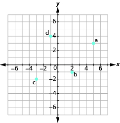
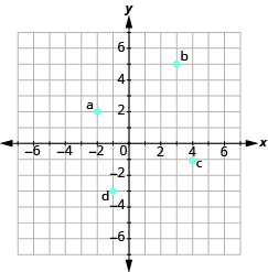
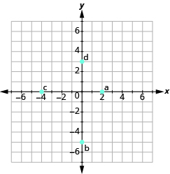
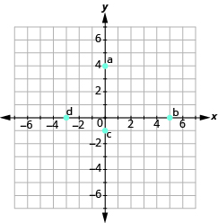
Identify Points on a Graph
In the following exercises, name the ordered pair of each point shown in the rectangular coordinate system.
Verify Solutions to an Equation in Two Variables
In the following exercises, find the ordered pairs that are solutions to the given equation.
- 5x + y = 10
- (5, 1)
- (2, 0)
- (4, −10)
- y = 6x − 2
- (1, 4)
- \(\left(\dfrac{1}{3} , 0\right)\)
- (6, −2)
Complete a Table of Solutions to a Linear Equation in Two Variables
In the following exercises, complete the table to find solutions to each linear equation.
- y = 4x − 1
| x | y | (x, y) |
|---|---|---|
| 0 | ||
| 1 | ||
| -2 |
- y = \(− \dfrac{1}{2}\)x + 3
| x | y | (x, y) |
|---|---|---|
| 0 | ||
| 1 | ||
| -2 |
- x + 2y = 5
| x | y | (x, y) |
|---|---|---|
| 0 | ||
| 1 | ||
| -1 |
- 3x − 2y = 6
| x | y | (x, y) |
|---|---|---|
| 0 | ||
| 0 | ||
| -2 |
Find Solutions to a Linear Equation in Two Variables
In the following exercises, find three solutions to each linear equation.
- x + y = 3
- x + y = −4
- y = 3x + 1
- y = − x − 1
11.2 - Graphing Linear Equations
Recognize the Relation Between the Solutions of an Equation and its Graph
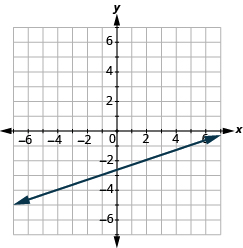
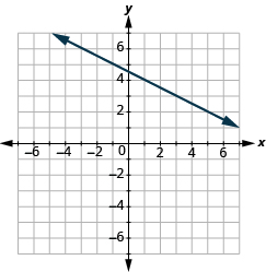
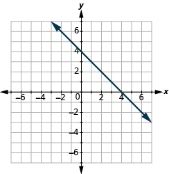
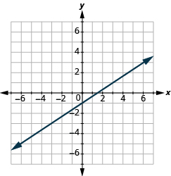
In the following exercises, for each ordered pair, decide (a) if the ordered pair is a solution to the equation. (b) if the point is on the line.
- y = − x + 4
- (0, 4)
- (−1, 3)
- (2, 2)
- (−2, 6)
- y = \(\dfrac{2}{3}\)x − 1
- (0, −1)
- (3, 1)
- (−3, −3)
- (6, 4)
Graph a Linear Equation by Plotting Points
In the following exercises, graph by plotting points.
- y = 4x − 3
- y = −3x
- 2x + y = 7
Graph Vertical and Horizontal lines
In the following exercises, graph the vertical or horizontal lines.
- y = −2
- x = 3
11.3 - Graphing with Intercepts
Identify the Intercepts on a Graph
In the following exercises, find the x- and y-intercepts.
Find the Intercepts from an Equation of a Line
In the following exercises, find the intercepts.
- x + y = 5
- x − y = −1
- y = \(\dfrac{3}{4}\)x − 12
- y = 3x
Graph a Line Using the Intercepts
In the following exercises, graph using the intercepts.
- −x + 3y = 3
- x + y = −2
Choose the Most Convenient Method to Graph a Line
In the following exercises, identify the most convenient method to graph each line.
- x = 5
- y = −3
- 2x + y = 5
- x − y = 2
- y = \(\dfrac{1}{2}\)x + 2
- y = \(\dfrac{3}{4}\)x − 1
11.4 - Understand Slope of a Line
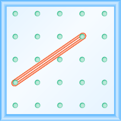
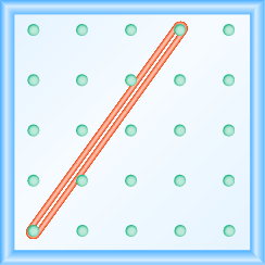
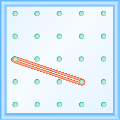
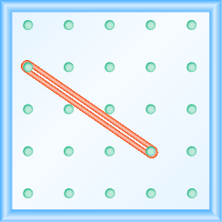
Use Geoboards to Model Slope
In the following exercises, find the slope modeled on each geoboard.
In the following exercises, model each slope. Draw a picture to show your results.
- \(\dfrac{1}{3}\)
- \(\dfrac{3}{2}\)
- \(− \dfrac{2}{3}\)
- \(− \dfrac{1}{2}\)
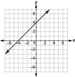
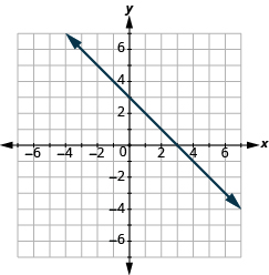
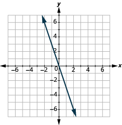
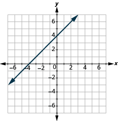
Find the Slope of a Line from its Graph
In the following exercises, find the slope of each line shown.
Find the Slope of Horizontal and Vertical Lines
In the following exercises, find the slope of each line.
- y = 2
- x = 5
- x = −3
- y = −1
Use the Slope Formula to find the Slope of a Line between Two Points
In the following exercises, use the slope formula to find the slope of the line between each pair of points.
- (2, 1), (4, 5)
- (−1, −1), (0, −5)
- (3, 5), (4, −1)
- (−5, −2), (3, 2)
Graph a Line Given a Point and the Slope
In the following exercises, graph the line given a point and the slope.
- (2, −2); m = \(\dfrac{5}{2}\)
- (−3, 4); m = \(− \dfrac{1}{3}\)
Solve Slope Applications
In the following exercise, solve the slope application.
- A roof has rise 10 feet and run 15 feet. What is its slope?
PRACTICE TEST
- Plot and label these points:
- (2, 5)
- (−1, −3)
- (−4, 0)
- (3, −5)
- (−2, 1)
- Name the ordered pair for each point shown.
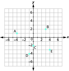
- Find the x-intercept and y-intercept on the line shown.
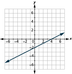
- Find the x-intercept and y-intercept of the equation 3x − y = 6.
- Is (1, 3) a solution to the equation x + 4y = 12? How do you know?
- Complete the table to find four solutions to the equation y = − x + 1.
| x | y | (x, y) |
|---|---|---|
| 0 | ||
| 1 | ||
| 3 | ||
| -2 |
- Complete the table to find three solutions to the equation 4x + y = 8.
| x | y | (x, y) |
|---|---|---|
| 0 | ||
| 0 | ||
| 3 |
In the following exercises, find three solutions to each equation and then graph each line.
- y = −3x
- 2x + 3y = −6
In the following exercises, find the slope of each line.
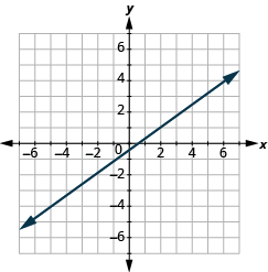
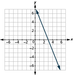
- Use the slope formula to find the slope of the line between (0, −4) and (5, 2).
- Find the slope of the line y = 2.
- Graph the line passing through (1, 1) with slope m = \(\dfrac{3}{2}\).
- A bicycle route climbs 20 feet for 1,000 feet of horizontal distance. What is the slope of the route?
Contributors and Attributions
Lynn Marecek (Santa Ana College) and MaryAnne Anthony-Smith (Formerly of Santa Ana College). This content is licensed under Creative Commons Attribution License v4.0 "Download for free at http://cnx.org/contents/fd53eae1-fa2...49835c3c@5.191."


