7.4: Modeling Changing Amplitude and Midline

Last updated
Save as PDF

Page ID: 13873

$ \newcommand{\vecs}[1]{\overset { \scriptstyle \rightharpoonup} {\mathbf{#1}} } $

$ \newcommand{\vecd}[1]{\overset{-\!-\!\rightharpoonup}{\vphantom{a}\smash {#1}}} $

$ \newcommand{\id}{\mathrm{id}}$ $ \newcommand{\Span}{\mathrm{span}}$

( \newcommand{\kernel}{\mathrm{null}\,}\) $ \newcommand{\range}{\mathrm{range}\,}$

$ \newcommand{\RealPart}{\mathrm{Re}}$ $ \newcommand{\ImaginaryPart}{\mathrm{Im}}$

$ \newcommand{\Argument}{\mathrm{Arg}}$ $ \newcommand{\norm}[1]{\| #1 \|}$

$ \newcommand{\inner}[2]{\langle #1, #2 \rangle}$

$ \newcommand{\Span}{\mathrm{span}}$

$ \newcommand{\id}{\mathrm{id}}$

$ \newcommand{\Span}{\mathrm{span}}$

$ \newcommand{\kernel}{\mathrm{null}\,}$

$ \newcommand{\range}{\mathrm{range}\,}$

$ \newcommand{\RealPart}{\mathrm{Re}}$

$ \newcommand{\ImaginaryPart}{\mathrm{Im}}$

$ \newcommand{\Argument}{\mathrm{Arg}}$

$ \newcommand{\norm}[1]{\| #1 \|}$

$ \newcommand{\inner}[2]{\langle #1, #2 \rangle}$

$ \newcommand{\Span}{\mathrm{span}}$ $ \newcommand{\AA}{\unicode[.8,0]{x212B}}$

$ \newcommand{\vectorA}[1]{\vec{#1}} % arrow$

$ \newcommand{\vectorAt}[1]{\vec{\text{#1}}} % arrow$

$ \newcommand{\vectorB}[1]{\overset { \scriptstyle \rightharpoonup} {\mathbf{#1}} } $

$ \newcommand{\vectorC}[1]{\textbf{#1}} $

$ \newcommand{\vectorD}[1]{\overrightarrow{#1}} $

$ \newcommand{\vectorDt}[1]{\overrightarrow{\text{#1}}} $

$ \newcommand{\vectE}[1]{\overset{-\!-\!\rightharpoonup}{\vphantom{a}\smash{\mathbf {#1}}}} $

$ \newcommand{\vecs}[1]{\overset { \scriptstyle \rightharpoonup} {\mathbf{#1}} } $

$ \newcommand{\vecd}[1]{\overset{-\!-\!\rightharpoonup}{\vphantom{a}\smash {#1}}} $

$\newcommand{\avec}{\mathbf a}$ $\newcommand{\bvec}{\mathbf b}$ $\newcommand{\cvec}{\mathbf c}$ $\newcommand{\dvec}{\mathbf d}$ $\newcommand{\dtil}{\widetilde{\mathbf d}}$ $\newcommand{\evec}{\mathbf e}$ $\newcommand{\fvec}{\mathbf f}$ $\newcommand{\nvec}{\mathbf n}$ $\newcommand{\pvec}{\mathbf p}$ $\newcommand{\qvec}{\mathbf q}$ $\newcommand{\svec}{\mathbf s}$ $\newcommand{\tvec}{\mathbf t}$ $\newcommand{\uvec}{\mathbf u}$ $\newcommand{\vvec}{\mathbf v}$ $\newcommand{\wvec}{\mathbf w}$ $\newcommand{\xvec}{\mathbf x}$ $\newcommand{\yvec}{\mathbf y}$ $\newcommand{\zvec}{\mathbf z}$ $\newcommand{\rvec}{\mathbf r}$ $\newcommand{\mvec}{\mathbf m}$ $\newcommand{\zerovec}{\mathbf 0}$ $\newcommand{\onevec}{\mathbf 1}$ $\newcommand{\real}{\mathbb R}$ $\newcommand{\twovec}[2]{\left[\begin{array}{r}#1 \\ #2 \end{array}\right]}$ $\newcommand{\ctwovec}[2]{\left[\begin{array}{c}#1 \\ #2 \end{array}\right]}$ $\newcommand{\threevec}[3]{\left[\begin{array}{r}#1 \\ #2 \\ #3 \end{array}\right]}$ $\newcommand{\cthreevec}[3]{\left[\begin{array}{c}#1 \\ #2 \\ #3 \end{array}\right]}$ $\newcommand{\fourvec}[4]{\left[\begin{array}{r}#1 \\ #2 \\ #3 \\ #4 \end{array}\right]}$ $\newcommand{\cfourvec}[4]{\left[\begin{array}{c}#1 \\ #2 \\ #3 \\ #4 \end{array}\right]}$ $\newcommand{\fivevec}[5]{\left[\begin{array}{r}#1 \\ #2 \\ #3 \\ #4 \\ #5 \\ \end{array}\right]}$ $\newcommand{\cfivevec}[5]{\left[\begin{array}{c}#1 \\ #2 \\ #3 \\ #4 \\ #5 \\ \end{array}\right]}$ $\newcommand{\mattwo}[4]{\left[\begin{array}{rr}#1 \amp #2 \\ #3 \amp #4 \\ \end{array}\right]}$ $\newcommand{\laspan}[1]{\text{Span}\{#1\}}$ $\newcommand{\bcal}{\cal B}$ $\newcommand{\ccal}{\cal C}$ $\newcommand{\scal}{\cal S}$ $\newcommand{\wcal}{\cal W}$ $\newcommand{\ecal}{\cal E}$ $\newcommand{\coords}[2]{\left\{#1\right\}_{#2}}$ $\newcommand{\gray}[1]{\color{gray}{#1}}$ $\newcommand{\lgray}[1]{\color{lightgray}{#1}}$ $\newcommand{\rank}{\operatorname{rank}}$ $\newcommand{\row}{\text{Row}}$ $\newcommand{\col}{\text{Col}}$ $\renewcommand{\row}{\text{Row}}$ $\newcommand{\nul}{\text{Nul}}$ $\newcommand{\var}{\text{Var}}$ $\newcommand{\corr}{\text{corr}}$ $\newcommand{\len}[1]{\left|#1\right|}$ $\newcommand{\bbar}{\overline{\bvec}}$ $\newcommand{\bhat}{\widehat{\bvec}}$ $\newcommand{\bperp}{\bvec^\perp}$ $\newcommand{\xhat}{\widehat{\xvec}}$ $\newcommand{\vhat}{\widehat{\vvec}}$ $\newcommand{\uhat}{\widehat{\uvec}}$ $\newcommand{\what}{\widehat{\wvec}}$ $\newcommand{\Sighat}{\widehat{\Sigma}}$ $\newcommand{\lt}{<}$ $\newcommand{\gt}{>}$ $\newcommand{\amp}{&}$ $\definecolor{fillinmathshade}{gray}{0.9}$

Section 7.4 Modeling Changing Amplitude and Midline

While sinusoidal functions can model a variety of behaviors, it is often necessary to combine sinusoidal functions with linear and exponential curves to model real applications and behaviors. We begin this section by looking at changes to the midline of a sinusoidal function. Recall that the midline describes the middle, or average value, of the sinusoidal function.

Changing Midlines

Example $\PageIndex{1}$

A population of elk currently averages 2000 elk, and that average has been growing by 4% each year. Due to seasonal fluctuation, the population oscillates from 50 below average in the winter up to 50 above average in the summer. Find a function that models the number of elk after $t$ years, starting in the winter.

Solution

There are two components to the behavior of the elk population: the changing average, and the oscillation. The average is an exponential growth, starting at 2000 and growing by 4% each year. Writing a formula for this:

\[average=initial(1+r)^{t} =2000(1+0.04)^{t}\nonumber\]

For the oscillation, since the population oscillates 50 above and below average, the amplitude will be 50. Since it takes one year for the population to cycle, the period is 1. We find the value of the horizontal stretch coefficient \[B=\frac{\text{original period}}{\text{new period}}=\frac{2\pi }{1}=2\pi \nonumber\]

The function starts in winter, so the shape of the function will be a negative cosine, since it starts at the lowest value.

Putting it all together, the equation would be:

\[P(t)=-50\cos (2\pi {\kern 1pt} t)+midline\nonumber\]

Since the midline represents the average population, we substitute in the exponential function into the population equation to find our final equation:

\[P(t)=-50\cos (2\pi {\kern 1pt} t)+2000(1+0.04)^{t}\nonumber\]

This is an example of changing midline – in this case an exponentially changing midline.

CHANGING MIDLINE

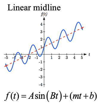
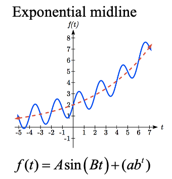
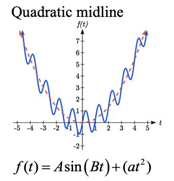
A function of the form $f(t)=A\sin (Bt)+g(t)$ will oscillate above and below the average given by the function $g(t)$.

Changing Midline

Changing midlines can be exponential, linear, or any other type of function. Here are some examples:

$A graph showing an increasing line in dashed red, with a sinusoidal-style function in blue shown oscillating above and below that line, with constant period, and peaks and valleys a constant distance above and below the line.$ $A graph showing an increasing exponential curve in dashed red, with a sinusoidal-style function in blue shown oscillating above and below that curve, with constant period, and peaks and valleys a constant distance above and below the curve.$ $A graph showing a U-shaped parabolic curve in dashed red, with a sinusoidal-style function in blue shown oscillating above and below that curve, with constant period, and peaks and valleys a constant distance above and below the curve.$

Example $\PageIndex{2}$

Find a function with linear midline of the form $f(t)=A\sin \left(\dfrac{\pi }{2} t\right)+mt+b$ that will pass through the points given below.

$t$	0	1	2	3
$f(t)$	5	10	9	8

Since we are given the value of the horizontal compression coefficient we can calculate the period of this function: new period = $\dfrac{\text{original period}}{B}$ = $\dfrac{2\pi}{\pi/2}$ = 4.

Solution

Since the sine function is at the midline at the beginning of a cycle and halfway through a cycle, we would expect this function to be at the midline at t = 0 and t = 2, since 2 is half the full period of 4. Based on this, we expect the points (0, 5) and (2, 9) to be points on the midline. We can clearly see that this is not a constant function and so we use the two points to calculate a linear function: $midline=mt+b$. From these two points we can calculate a slope:

\[m=\dfrac{9-5}{2-0} =\dfrac{4}{2} =2\nonumber\]

Combining this with the initial value of 5, we have the midline: $midline=2t+5$.

The full function will have form $f(t)=A\sin \left(\dfrac{\pi }{2} t\right)+2t+5$. To find the amplitude, we can plug in a point we haven’t already used, such as (1, 10).

\[10=A\sin \left(\dfrac{\pi }{2} (1)\right)+2(1)+5\nonumber\]Evaluate the sine and combine like terms
\[10=A+7\nonumber\]
\[A=3\nonumber\]

A function of the form given fitting the data would be

\[f(t)=3\sin \left(\dfrac{\pi }{2} t\right)+2t+5\nonumber\]

Notice we could have taken an alternate approach by plugging points (0, 5) and (2, 9) into the original equation. Substituting (0, 5),

\[5=A\sin \left(\dfrac{\pi }{2} (0)\right)+m(0)+b\nonumber\]Evaluate the sine and simplify
\[5=b\nonumber\]

Substituting (2, 9)

\[9=A\sin \left(\dfrac{\pi }{2} (2)\right)+m(2)+5\nonumber\]Evaluate the sine and simplify
\[9=2m+5\nonumber\]
\[4=2m\nonumber\]
\[m=2\nonumber\]as we found above. Now we can proceed to find $A$ the same way we did before.

Example $\PageIndex{3}$

The number of tourists visiting a ski and hiking resort averages 4000 people annually and oscillates seasonally, 1000 above and below the average. Due to a marketing campaign, the average number of tourists has been increasing by 200 each year. Write an equation for the number of tourists after $t$ years, beginning at the peak season.

$A graph showing a dashed line in red that starts at 0 comma 4000 and passes through 5 comma 5000. A sinusoidal-style function is shown in blue, with peaks and valleys staing a constant amplitude above and below the line. It starts above the red line at 0 comma 5000, decreasing below the line, then increasing back up to another high at 1 comma 5200.$

Solution

Again there are two components to this problem: the oscillation and the average. For the oscillation, the number of tourists oscillates 1000 above and below average, giving an amplitude of 1000. Since the oscillation is seasonal, it has a period of 1 year. Since we are given a starting point of “peak season”, we will model this scenario with a cosine function.

So far, this gives an equation in the form $N(t)=1000\cos (2\pi {\kern 1pt} t)+midline$.

The average is currently 4000, and is increasing by 200 each year. This is a constant rate of change, so this is linear growth, $average=4000+200t$. This function will act as the midline.

Combining these two pieces gives a function for the number of tourists:

\[N(t)=1000\cos (2\pi {\kern 1pt} t)+4000+200t\nonumber\]

Exercise $\PageIndex{1}$

Given the function $g(x)=(x^{2} -1)+8\cos (x)$, describe the midline and amplitude using words.

Answer: The midline follows the path of the quadratic $x^{2} -1$ and the amplitude is a constant value of 8.

Changing Amplitude

There are also situations in which the amplitude of a sinusoidal function does not stay constant. Back in Chapter 6, we modeled the motion of a spring using a sinusoidal function, but had to ignore friction in doing so. If there were friction in the system, we would expect the amplitude of the oscillation to decrease over time. In the equation $f(t)=A\sin (Bt)+k$, $A$ gives the amplitude of the oscillation, we can allow the amplitude to change by replacing this constant $A$ with a function $A(t)$.

CHANGING AMPLITUDE

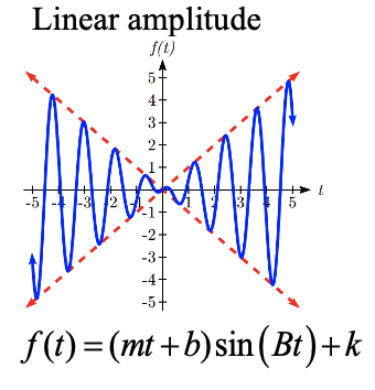
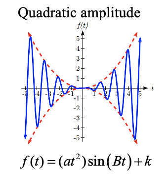
A function of the form $f(t)=A(t)\sin (Bt)+k$ will oscillate above and below the midline with an amplitude given by $A(t)$.

Here are some examples:

$A graph showing two dashed lines in red, an increasing y equals t graph, and a decreasing y equals negative t graph, crossing at the origin. A sinusoidal-style function is shown in blue, with constant period, midline at 0, and amplitude changing so the peaks and valleys touch the two dashed lines.$ $A graph showing two dashed curves in red, an increasing concave up exponential graph, and it's vertical reflection. A sinusoidal-style function is shown in blue, with constant period, midline at 0, and amplitude changing so the peaks and valleys touch the two dashed curves.$ $A graph showing two dashed curves in red, an upwards-opening U-shaped parabolic graph of y equals x squared, and it's vertical reflection. A sinusoidal-style function is shown in blue, with constant period, midline at 0, and amplitude changing so the peaks and valleys touch the two dashed curves.$

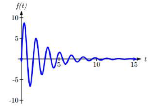
When thinking about a spring with amplitude decreasing over time, it is tempting to use the simplest tool for the job – a lin $A sinusoidal-style graph with constant period and midline at 0, which starts with an amplitude of 10 which decreases linearly to an amplitude of 0 when t equals 10. The amplitude then increases linearly.$ ear function. But if we attempt to model the amplitude with a decreasing linear function, such as $A(t)=10-t$, we quickly see the problem when we graph the equation $f(t)=(10-t)\sin (4t)$.

While the amplitude decreases at first as intended, the amplitude hits zero at $t = 10$, then continues past the intercept, increasing in absolute value, which is not the expected behavior. This behavior and function may model the situation on a restricted domain and we might try to chalk the rest of it up to model breakdown, but in fact springs just don’t behave like this.

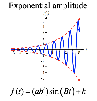
$A sinusoidal-style graph with constant period and midline at 0, which starts with an amplitude of 10 which decreases exponentially, approaching 0 as t approaches infinity.$

A better model, as you will learn later in physics and calculus, would show the amplitude decreasing by a fixed percentage each second, leading to an exponential decay model for the amplitude.

DAMPED HARMONIC MOTION

Damped harmonic motion, exhibited by springs subject to friction, follows a model of the form

\[f(t)=ab^{t} \sin (Bt)+k\text{ or }f(t)=ae^{rt} \sin (Bt)+k\nonumber\]

Example $\PageIndex{4}$

A spring with natural length of feet inches is pulled back 6 feet and released. It oscillates once every 2 seconds. Its amplitude decreases by 20% each second. Find a function that models the position of the spring t seconds after being released.

Solution

Since the spring will oscillate on either side of the natural length, the midline will be at 20 feet. The oscillation has a period of 2 seconds, and so the horizontal compression coefficient is $B=\pi$. Additionally, it begins at the furthest distance from the wall, indicating a cosine model.

$A sinusoidal-style graph that hits a peak at t equals 0, 2, 4, etc. The graph oscillates above and below a midline of y equals 20. The graph starts at 0 comma 26, decreases down to 1 comma about 15, increases to 2 comma about 24, decreases to 3 comma 17, and continues to oscillate with decreasing amplitude.$ Meanwhile, the amplitude begins at 6 feet, and decreases by 20% each second, giving an amplitude function of $A(t)=6(1-0.20)^{t}$.

Combining this with the sinusoidal information gives a function for the position of the spring:

\[f(t)=6(0.80)^{t} \cos (\pi {\kern 1pt} t)+20\nonumber\]

Example $\PageIndex{5}$

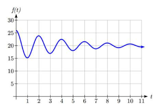
A spring with natural length of 30 cm is pulled out 10 cm and released. It oscillates 4 times per second. After 2 seconds, the amplitude has decreased to 5 cm. Find a function that models the position of the spring.

Solution

The oscillation has a period of $\dfrac{1}{4}$ second, so $B = \dfrac{2\pi}{1/4} = 8\pi$. Since the spring will oscillate on either side of the natural length, the midline will be at 30 cm. It begins at the furthest distance from the wall, suggesting a cosine model. Together, this gives

\[f(t)=A(t)\cos (8\pi {\kern 1pt} t)+30.\nonumber\]

For the amplitude function, we notice that the amplitude starts at 10 cm, and decreases to 5 cm after 2 seconds. This gives two points (0, 10) and (2, 5) that must be satisfied by an exponential function: $A(0)=10$ and $A(2)=5$. Since the function is exponential, we can use the form $A(t)=ab^{t}$. Substituting the first point, $10=ab^{0}$, so $a = 10$. Substituting in the second point,

\[5=10b^{2}\nonumber\]Divide by 10
\[\dfrac{1}{2} =b^{2}\nonumber\]Take the square root
\[b=\sqrt{\dfrac{1}{2} } \approx 0.707\nonumber\]

This gives an amplitude function of $A(t)=10(0.707)^{t}$. Combining this with the oscillation,

\[f(t)=10(0.707)^{t} \cos (8\pi t)+30\nonumber\]

Exercise $\PageIndex{2}$

A certain stock started at a high value of $7 per share, oscillating monthly above and below the average value, with the oscillation decreasing by 2% per year. However, the average value started at $4 per share and has grown linearly by 50 cents per year.

a. Find a formula for the midline and the amplitude.
b. Find a function $S(t)$ that models the value of the stock after $t$ years.

Answer: \[\begin{array}{l} {m(t)=4+0.5t} \\ {A(t)=7(0.98)^{t} } \end{array}\nonumber\]
\[S(t)= 7(0.98)^{t} \cos \left(24\pi t\right)+4+0.5t\nonumber\]

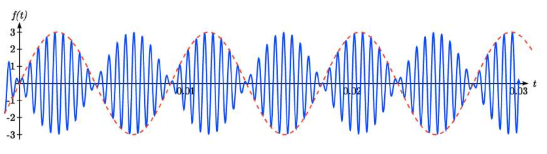
Example $\PageIndex{6}$

In AM (Amplitude Modulated) radio, a carrier wave with a high frequency is used to transmit music or other signals by applying the to-be-transmitted signal as the amplitude of the carrier signal. A musical note with frequency 110 Hz (Hertz = cycles per second) is to be carried on a wave with frequency of 2 KHz (KiloHertz = thousands of cycles per second). If the musical wave has an amplitude of 3, write a function describing the broadcast wave.

Solution

The carrier wave, with a frequency of 2000 cycles per second, would have period $\dfrac{1}{2000}$ of a second, giving an equation of the form $\sin (4000\pi {\kern 1pt} t)$. Our choice of a sine function here was arbitrary – it would have worked just was well to use a cosine.

The musical tone, with a frequency of 110 cycles per second, would have a period of $\dfrac{1}{110}$ of a second. With an amplitude of 3, this would correspond to a function of the form $3\sin (220\pi {\kern 1pt} t)$. Again our choice of using a sine function is arbitrary.

The musical wave is acting as the amplitude of the carrier wave, so we will multiply the musical tone’s function by the carrier wave function, resulting in the function

\[f(t)=3\sin (220\pi {\kern 1pt} t)\sin (4000\pi {\kern 1pt} t)\nonumber\]

$Three cycles of a sine graph are shown dashed in red, with a period of 1 over 110. A much higher frequency sinusoidal-style curve is shown in blue, with a period of 1 over 2000, with a midline at 0, and the peaks and valleys of the curve touching the dashed sine curve and its vertical reflection.$

Important Topics of This Section

Changing midline
Changing amplitude
Linear Changes
Exponential Changes
Damped Harmonic Motion

Search

Text Color

Text Size

Margin Size

Font Type

\(t\)	0	1	2	3
\(f(t)\)	5	10	9	8