3.2: Transformations of Common Graphs

Last updated
Save as PDF

Page ID: 83123

$ \newcommand{\vecs}[1]{\overset { \scriptstyle \rightharpoonup} {\mathbf{#1}} } $ $ \newcommand{\vecd}[1]{\overset{-\!-\!\rightharpoonup}{\vphantom{a}\smash {#1}}} $$\newcommand{\id}{\mathrm{id}}$ $ \newcommand{\Span}{\mathrm{span}}$ $ \newcommand{\kernel}{\mathrm{null}\,}$ $ \newcommand{\range}{\mathrm{range}\,}$ $ \newcommand{\RealPart}{\mathrm{Re}}$ $ \newcommand{\ImaginaryPart}{\mathrm{Im}}$ $ \newcommand{\Argument}{\mathrm{Arg}}$ $ \newcommand{\norm}[1]{\| #1 \|}$ $ \newcommand{\inner}[2]{\langle #1, #2 \rangle}$ $ \newcommand{\Span}{\mathrm{span}}$ $\newcommand{\id}{\mathrm{id}}$ $ \newcommand{\Span}{\mathrm{span}}$ $ \newcommand{\kernel}{\mathrm{null}\,}$ $ \newcommand{\range}{\mathrm{range}\,}$ $ \newcommand{\RealPart}{\mathrm{Re}}$ $ \newcommand{\ImaginaryPart}{\mathrm{Im}}$ $ \newcommand{\Argument}{\mathrm{Arg}}$ $ \newcommand{\norm}[1]{\| #1 \|}$ $ \newcommand{\inner}[2]{\langle #1, #2 \rangle}$ $ \newcommand{\Span}{\mathrm{span}}$$\newcommand{\AA}{\unicode[.8,0]{x212B}}$

The transformation of graphs, using common functions, will be a skill that will bring insight to graphing functions quickly and painlessly. Anticipating how a graph of a function will look, and transforming old graphs to new graphs, is a skill we will explore in this section. Mastering this skill will give you a leg up on understanding analytic geometry, a key component to calculus.

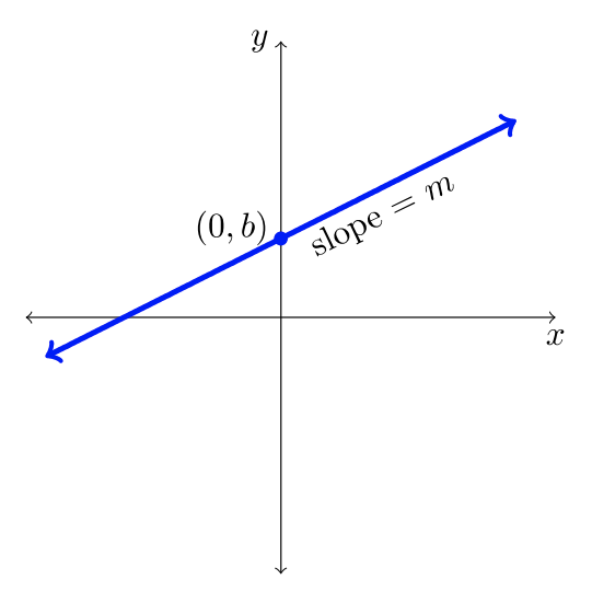
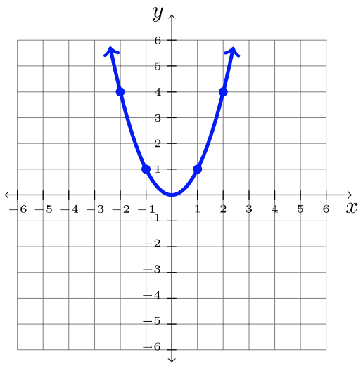
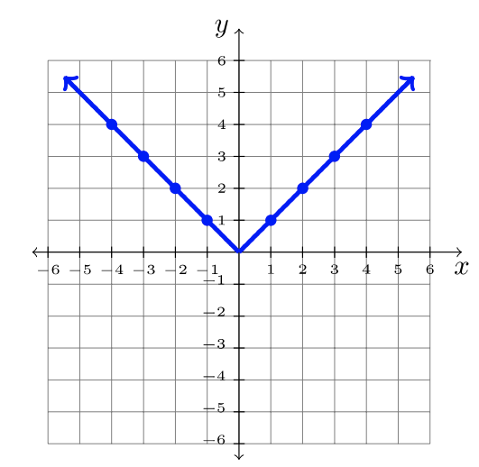
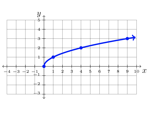
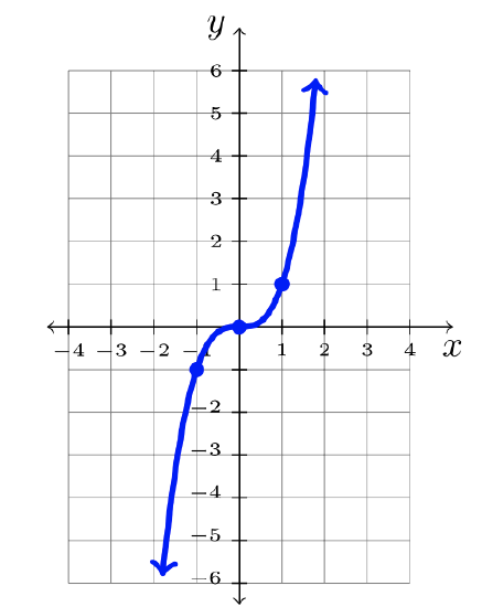
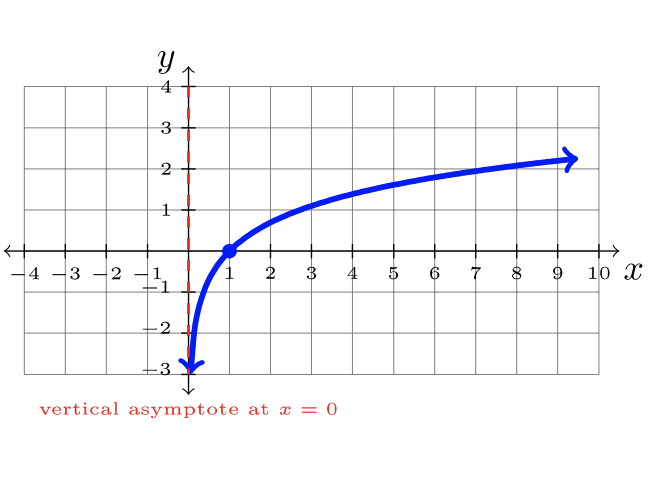
Here are nine common functions and their graphs. Each of these functions will be referred to as “the parent function” for its family of transformed functions.

$f(x) = mx + b$	$f(x) = x^2$	$f(x) = \|x\|$
$clipboard_e0ec7b4b76f35f18f5c5d52c9eee803a0.png$	$clipboard_e1f6b7583bfa4bfd9e900f971f6326904.png$	$clipboard_eb5265d3568b1bde6688a1643e83fbb2f.png$

$f(x) = \sqrt{x}$	$f(x) = x^3$	$f(x) = \ln x$
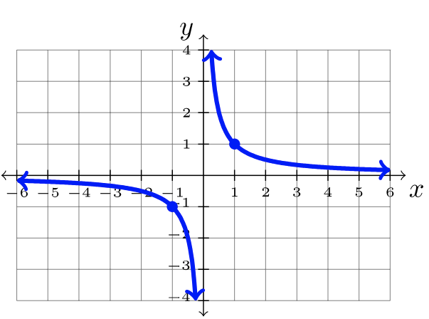
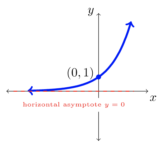
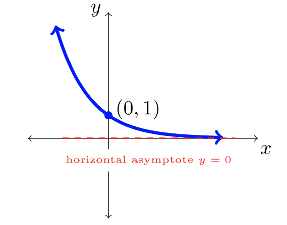
$clipboard_ea79b8b364466de80daf366ac9f77a213.png$	$clipboard_eb696b0dbf8723799beac338367bff4f6.png$	$clipboard_ef55d89ef8d0d94dc91394b9c6ce3e140.png$

$f(x) = \dfrac{1}{x}$	$f(x) = b^x$ where $b>1$	$f(x) = b^x$ where $0 < b< 1$
$clipboard_ee226d5b5690b009e6046c50cb7d2d5c0.png$	$clipboard_e583f09166f4bbaa71c9fd4593537850a.png$	$clipboard_e87fce111b41fff6ce78cf7158cf79a37.png$

Using the transformations described in Section $3.1$, the nine graphs shown on the previous page can be shifted, reflected, stretched, and compressed. The take-away for this section is to recognize the parent function from function notation and apply the appropriate transformations to quickly sketch a graph or visualize the graph in your head. No technology is necessary! It’s enough to have an understanding for functions and their shifting graphs.

Example 3.2.1

Name the parent function of the given function. Then describe in words the transformation(s) on the parent function.

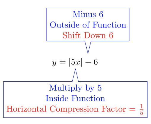
$y = |5x| − 6$
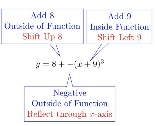
$y = 8 − (x + 9)^3$
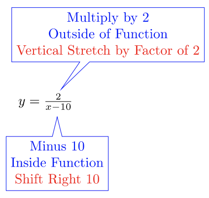
$y = \dfrac{2}{x−10}$

Solution

The parent function is $y = |x|$:

$clipboard_ebfa3193f5b191a25838e1d453b7ad2f1.png$

The parent function is $y = x^3$:

$clipboard_e3e89bc7a9522c97737286bda529f642d.png$

The parent function is $y = \dfrac{1}{x}$:

$clipboard_e4fce349c053cbf533b9a2e3b49ca5f0e.png$

Example 3.2.2

Use the parent function and its transformation(s) to sketch the graph of the given function. It is much more important to create a rough but accurate sketch without technology than a detailed sketch with technology.

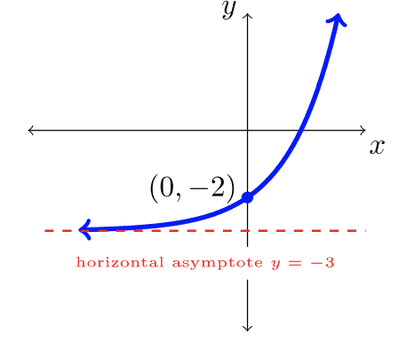
$y = 2^x − 3$
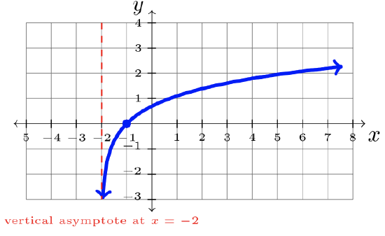
$y = \ln(x + 2)$

Solution

The parent function is $y = b^x$ where $b = 2 > 1$. Shift this graph, including its horizontal asymptote, down $3$ units.

$clipboard_e81c6d4d163303c1fc1bd59a171d63ef5.png$

The parent function is $y = \ln x$. Shift this graph, including its vertical asymptote, left $2$ units.

$clipboard_e284658bbaaa0722df9427746025c760b.png$

Try It! (Exercises)

For exercises #1-18, use the parent functions (see graphs within this section), along with appropriate transformations, to create a sketch of the graph of the given function. Do not use graphing technology.

$y = \dfrac{1}{x+5}$
$y = e^{x−4}$
$y = |x| − 6$
$y = −(x + 2)^3$
$y = 4 + x^2$
$y = \sqrt{x − 4}$
$y = \left( \dfrac{1}{2} \right)^x + 3$
$y = 1 − \sqrt{x}$
$y = |x − 5| + 2$
$y = 1 + (x − 6)^2$
$y = 4 − \dfrac{1}{x}$
$y = 3 + \ln (−x)$
$y = 2\sqrt{x} − 4$
$y = −2(x − 5)^2$
$y = 1 + x^3$
$y = −3|x − 7|$
$y = 5 + \sqrt{-x}$
$y= 3^{x+2} + 4$
Use the graph of $y = |x|$ and transformations to discuss why the graph of the transformed function $y = |-x|$ is the same graph.
Use the graph of $y = x^2$ and transformations to discuss why the graph of the transformed function $y = (-x)^2$ is the same graph.
Using $f(x) = x^2$ as the parent function, write the function that would correspond to the transformations on $f$. No need to graph.

a. Reflected through the $x$-axis and shifted down $12$ units.

b. Shifted $10$ units left and $25$ units up.

Discuss two different approaches to transform the parent function $y = \dfrac{1}{x}$ to graph $y = \dfrac{1}{2x}$. What are the transformations? Discuss how and why each approach will produce the same graph for the new function $y = \dfrac{1}{2x}$.

\(f(x) = mx + b\)	\(f(x) = x^2\)	\(f(x) = \|x\|\)
$clipboard_e0ec7b4b76f35f18f5c5d52c9eee803a0.png$	$clipboard_e1f6b7583bfa4bfd9e900f971f6326904.png$	$clipboard_eb5265d3568b1bde6688a1643e83fbb2f.png$

\(f(x) = \sqrt{x}\)	\(f(x) = x^3\)	\(f(x) = \ln x\)
$clipboard_ea79b8b364466de80daf366ac9f77a213.png$	$clipboard_eb696b0dbf8723799beac338367bff4f6.png$	$clipboard_ef55d89ef8d0d94dc91394b9c6ce3e140.png$

\(f(x) = \dfrac{1}{x}\)	\(f(x) = b^x\) where \(b>1\)	\(f(x) = b^x\) where \(0 < b< 1\)
$clipboard_ee226d5b5690b009e6046c50cb7d2d5c0.png$	$clipboard_e583f09166f4bbaa71c9fd4593537850a.png$	$clipboard_e87fce111b41fff6ce78cf7158cf79a37.png$