5.3: Inverse Trigonometric Functions

We have briefly mentioned the inverse trigonometric functions before, for example in Section 1.3 when we discussed how to use the $\fbox{\(\sin^{-1}\)}$, $\fbox{\(\cos^{-1}\)}$, and $\fbox{\(\tan^{-1}\)}$ buttons on a calculator to find an angle that has a certain trigonometric function value. We will now define those inverse functions and determine their graphs.

Figure 5.3.1

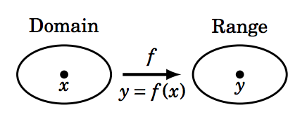
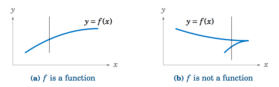
Recall that a function is a rule that assigns a single object $y$ from one set (the range to each object $x$ from another set (the domain). We can write that rule as $y = f(x)$, where $f$ is the function (see Figure 5.3.1). There is a simple vertical rule for determining whether a rule $y=f(x)$ is a function: $f$ is a function if and only if every vertical line intersects the graph of $y=f(x)$ in the $xy$-coordinate plane at most once (see Figure 5.3.2).

Figure 5.3.2 Vertical rule for functions

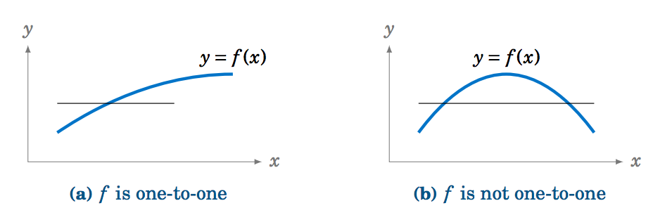
Recall that a function $f$ is one-to-one (often written as $1-1$) if it assigns distinct values of $y$ to distinct values of $x$. In other words, if $x_1 \ne x_2$ then $f(x_1 ) \ne f(x_2 )$. Equivalently, $f$ is one-to-one if $f(x_1 ) = f(x_2 )$ implies $x_1 = x_2$. There is a simple horizontal rule for determining whether a function $y=f(x)$ is one-to-one: $f$ is one-to-one if and only if every horizontal line intersects the graph of $y=f(x)$ in the $xy$-coordinate plane at most once (see Figure 5.3.3).

Figure 5.3.3 Horizontal rule for one-to-one functions

If a function $f$ is one-to-one on its domain, then $f$ has an inverse function, denoted by $f^{-1}$, such that $y=f(x)$ if and only if $f^{-1}(y) = x$. The domain of $f^{-1}$ is the range of $f$.

The basic idea is that $f^{-1}$ "undoes'' what $f$ does, and vice versa. In other words,

$$\nonumber \begin{alignat*}{3} f^{-1}(f(x)) ~&=~ x \quad&&\text{for all \(x \) in the domain of \(f \), and}\\ \nonumber f(f^{-1}(y)) ~&=~ y \quad&&\text{for all \(y \) in the range of \(f \).} \end{alignat*} \nonumber$$

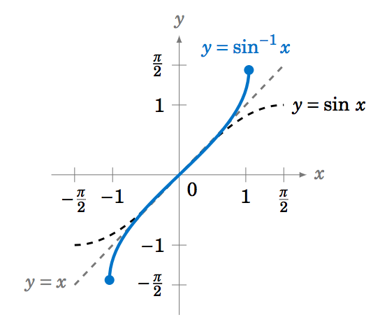
We know from their graphs that none of the trigonometric functions are one-to-one over their entire domains. However, we can restrict those functions to subsets of their domains where they are one-to-one. For example, $y=\sin\;x$ is one-to-one over the interval $\left[ -\frac{\pi}{2},\frac{\pi}{2} \right]$, as we see in the graph below:

Figure 5.3.4 $y = \sin x$ with $x$ restricted to $\left [ − \frac{π}{ 2} , \frac{π}{ 2} \right ]$

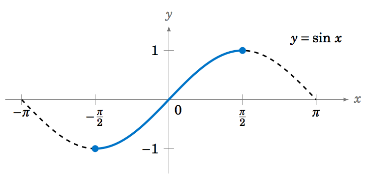
For $-\frac{\pi}{2} \le x \le \frac{\pi}{2}$ we have $-1 \le \sin\;x \le 1$, so we can define the inverse sine function $y=\sin^{-1} x$ (sometimes called the arc sine and denoted by $y=\arcsin\;x$) whose domain is the interval $[-1,1]$ and whose range is the interval $\left[ -\frac{\pi}{2},\frac{\pi}{2} \right]$. In other words:

$$\begin{alignat}{3} \sin^{-1} (\sin\;y) ~&=~ y \quad&&\text{for \(-\tfrac{\pi}{2} \le y \le \tfrac{\pi}{2}\)}\label{eqn:arcsin1}\\ \sin\;(\sin^{-1} x) ~&=~ x \quad&&\text{for \(-1 \le x \le 1\)}\label{eqn:arcsin2} \end{alignat} \nonumber$$

Example 5.13

Find $\sin^{-1} \left(\sin\;\frac{\pi}{4}\right)$.

Solution

Since $-\frac{\pi}{2} \le \frac{\pi}{4} \le \frac{\pi}{2}$, we know that $\sin^{-1} \left(\sin\;\frac{\pi}{4}\right) = \boxed{\frac{\pi}{4}}\;$, by Equation $\ref{eqn:arcsin1}$.

Example 5.14

Find $\sin^{-1} \left(\sin\;\frac{5\pi}{4}\right)$.

Solution

Since $\frac{5\pi}{4} > \frac{\pi}{2}$, we can not use Equation $\ref{eqn:arcsin1}$. But we know that $\sin\;\frac{5\pi}{4} = -\frac{1}{\sqrt{2}}$. Thus, $\sin^{-1} \left(\sin\;\frac{5\pi}{4}\right) = \sin^{-1} \left( -\frac{1}{\sqrt{2}} \right)$ is, by definition, the angle $y$ such that $-\frac{\pi}{2} \le y \le \frac{\pi}{2}$ and $\sin\;y = -\frac{1}{\sqrt{2}}$. That angle is $y=-\frac{\pi}{4}$, since

$$\sin\;\left( -\tfrac{\pi}{4} \right) ~=~ -\sin\;\left( \tfrac{\pi}{4} \right) ~=~ -\tfrac{1}{\sqrt{2}} ~. \nonumber$$

Thus, $\sin^{-1} \left(\sin\;\frac{5\pi}{4}\right) = \boxed{-\tfrac{\pi}{4}}\;$.

Example 5.14 illustrates an important point: $\sin^{-1} x$ should always be a number between $-\frac{\pi}{2}$ and $\frac{\pi}{2}$. If you get a number outside that range, then you made a mistake somewhere. This why in Example 1.27 in Section 1.5 we got $\sin^{-1}(-0.682) = -43^\circ$ when using the $\fbox{\(\sin^{-1}\)}$ button on a calculator. Instead of an angle between $0^\circ$ and $360^\circ$ (i.e. $0$ to $2\pi$ radians) we got an angle between $-90^\circ$ and $90^\circ$ (i.e. $-\frac{\pi}{2}$ to $\frac{\pi}{2}$ radians).

In general, the graph of an inverse function $f^{-1}$ is the reflection of the graph of $f$ around the line $y=x$. The graph of $y=\sin^{-1} x$ is shown in Figure 5.3.5. Notice the symmetry about the line $y=x$ with the graph of $y=\sin\;x$.

Figure 5.3.5 Graph of $y = \sin^{−1} x$

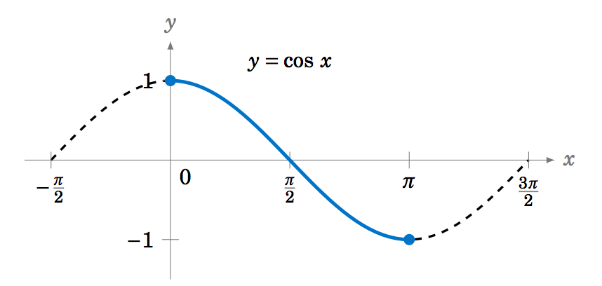
The inverse cosine function $y=\cos^{-1} x$ (sometimes called the arc cosine and denoted by $y=\arccos\;x$) can be determined in a similar fashion. The function $y=\cos\;x$ is one-to-one over the interval $[0,\pi]$, as we see in the graph below:

Figure 5.3.6 $y = \cos x$ with $x$ restricted to $[0,π]$

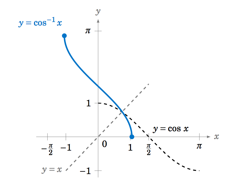
Thus, $y=\cos^{-1} x$ is a function whose domain is the interval $[-1,1]$ and whose range is the interval $[0,\pi]$. In other words:

$$\begin{alignat}{3} \cos^{-1} (\cos\;y) ~&=~ y \quad&&\text{for \(0 \le y \le \pi\)}\label{eqn:arccos1}\\ \cos\;(\cos^{-1} x) ~&=~ x \quad&&\text{for \(-1 \le x \le 1\)}\label{eqn:arccos2} \end{alignat} \nonumber$$

The graph of $y=\cos^{-1} x$ is shown below in Figure 5.3.7. Notice the symmetry about the line $y=x$ with the graph of $y=\cos\;x$.

Figure 5.3.7 Graph of $y = \cos^{−1} x$

Example 5.15

Find $\cos^{-1} \left(\cos\;\frac{\pi}{3}\right)$.

Solution

Since $0 \le \frac{\pi}{3} \le \pi$, we know that $\cos^{-1} \left(\cos\;\frac{\pi}{3}\right) = \boxed{\frac{\pi}{3}}\;$, by Equation $\ref{eqn:arccos1}$.

Example 5.16

Find $\cos^{-1} \left(\cos\;\frac{4\pi}{3}\right)$.

Solution

Since $\frac{4\pi}{3} > \pi$, we can not use Equation $\ref{eqn:arccos1}$. But we know that $\cos\;\frac{4\pi}{3} = -\frac{1}{2}$. Thus, $\cos^{-1} \left(\cos\;\frac{4\pi}{3}\right) = \cos^{-1} \left( -\frac{1}{2} \right)$ is, by definition, the angle $y$ such that $0 \le y \le \pi$ and $\cos\;y = -\frac{1}{2}$. That angle is $y=\frac{2\pi}{3}$ (i.e. $120^\circ$). Thus, $\cos^{-1} \left(\cos\;\frac{4\pi}{3}\right) = \boxed{\tfrac{2\pi}{3}}\;$.

Examples 5.14 and 5.16 may be confusing, since they seem to violate the general rule for inverse functions that $f^{-1}(f(x)) = x$ for all $x$ in the domain of $f$. But that rule only applies when the function $f$ is one-to-one over its entire domain. We had to restrict the sine and cosine functions to very small subsets of their entire domains in order for those functions to be one-to-one. That general rule, therefore, only holds for $x$ in those small subsets in the case of the inverse sine and inverse cosine.

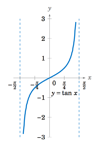
The inverse tangent function $y=\tan^{-1} x$ (sometimes called the arc tangent and denoted by $y=\arctan\;x$) can be determined similarly. The function $y=\tan\;x$ is one-to-one over the interval $\left( -\frac{\pi}{2},\frac{\pi}{2} \right)$, as we see in Figure 5.3.8:

Figure 5.3.8 $y = \tan x \text{ with }x \text{ restricted to }\left ( − \frac{π}{ 2} , \frac{π}{ 2} \right )$

The graph of $y=\tan^{-1} x$ is shown below in Figure 5.3.9. Notice that the vertical asymptotes for $y=\tan\;x$ become horizontal asymptotes for $y=\tan^{-1} x$. Note also the symmetry about the line $y=x$ with the graph of $y=\tan\;x$.

Figure 5.3.9 Graph of $y = \tan^{−1} x$

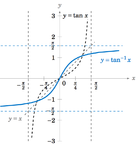
Thus, $y=\tan^{-1} x$ is a function whose domain is the set of all real numbers and whose range is the interval $\left( -\frac{\pi}{2},\frac{\pi}{2} \right)$. In other words:

$$\begin{alignat}{3} \tan^{-1} (\tan\;y) ~&=~ y \quad&&\text{for \(-\tfrac{\pi}{2} < y < \tfrac{\pi}{2}\)}\label{eqn:arctan1}\\ \tan\;(\tan^{-1} x) ~&=~ x \quad&&\text{for all real \(x\)}\label{eqn:arctan2} \end{alignat} \nonumber$$

Example 5.17

Find $\tan^{-1} \left(\tan\;\frac{\pi}{4}\right)$.

Solution

Since $-\tfrac{\pi}{2} \le \tfrac{\pi}{4} \le \tfrac{\pi}{2}$, we know that $\tan^{-1} \left(\tan\;\frac{\pi}{4}\right) = \boxed{\frac{\pi}{4}}\;$, by Equation $\ref{eqn:arctan1}$.

Example 5.18

Find $\tan^{-1} \left(\tan\;\pi\right)$.

Solution

Since $\pi > \tfrac{\pi}{2}$, we can not use Equation $\ref{eqn:arctan1}$. But we know that $\tan\;\pi = 0$. Thus, $\tan^{-1} \left(\tan\;\pi\right) = \tan^{-1} 0$ is, by definition, the angle $y$ such that $-\tfrac{\pi}{2} \le y \le \tfrac{\pi}{2}$ and $\tan\;y = 0$. That angle is $y=0$. Thus, $\tan^{-1} \left(\tan\;\pi \right) = \boxed{0}\;$.

Example 5.19

Find the exact value of $\cos\;\left(\sin^{-1}\;\left(-\frac{1}{4}\right)\right)$.

Solution

Let $\theta = \sin^{-1}\;\left(-\frac{1}{4}\right)$. We know that $-\tfrac{\pi}{2} \le \theta \le \tfrac{\pi}{2}$, so since $\sin\;\theta = -\frac{1}{4} < 0$, $\theta$ must be in QIV. Hence $\cos\;\theta > 0$. Thus,

$$\cos^2 \;\theta ~=~ 1 ~-~ \sin^2 \;\theta ~=~ 1 ~-~ \left( -\frac{1}{4} \right)^2 ~=~\frac{15}{16} \quad\Rightarrow\quad \cos\;\theta ~=~ \frac{\sqrt{15}}{4} ~. \nonumber$$

Note that we took the positive square root above since $\cos\;\theta > 0$. Thus, $\cos\;\left(\sin^{-1}\;\left(-\frac{1}{4}\right)\right) = \boxed{\frac{\sqrt{15}}{4}}\;$.

Example 5.20

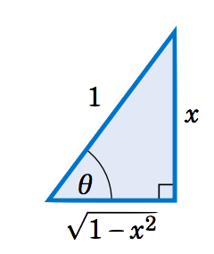
Show that $\tan\;(\sin^{-1} x) = \dfrac{x}{\sqrt{1 - x^2}}$ for $-1 < x < 1$.

Solution

When $x=0$, the Equation holds trivially, since

$$\nonumber \tan\;(\sin^{-1} 0) ~=~ \tan\;0 ~=~ 0 ~=~ \dfrac{0}{\sqrt{1 - 0^2}} ~. \nonumber$$

Now suppose that $0 < x < 1$. Let $\theta = \sin^{-1} x$. Then $\theta$ is in QI and $\sin\;\theta = x$. Draw a right triangle with an angle $\theta$ such that the opposite leg has length $x$ and the hypotenuse has length $1$, as in Figure 5.3.10 (note that this is possible since $0 < x < 1$). Then $\sin\;\theta = \frac{x}{1} = x$. By the Pythagorean Theorem, the adjacent leg has length $\sqrt{1 - x^2}$. Thus, $\tan\;\theta = \frac{x}{\sqrt{1 - x^2}}$.

Figure 5.3.10

If $-1 < x < 0$ then $\theta = \sin^{-1} x$ is in QIV. So we can draw the same triangle except that it would be "upside down'' and we would again have $\tan\;\theta = \frac{x}{\sqrt{1 - x^2}}$, since the tangent and sine have the same sign (negative) in QIV. Thus, $\tan\;(\sin^{-1} x) = \dfrac{x}{\sqrt{1 - x^2}}$ for $-1 < x < 1$.

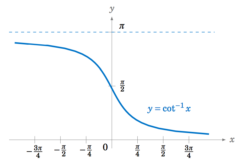
The inverse functions for cotangent, cosecant, and secant can be determined by looking at their graphs. For example, the function $y=\cot\;x$ is one-to-one in the interval $(0,\pi)$, where it has a range equal to the set of all real numbers. Thus, the inverse cotangent $y=\cot^{-1} x$ is a function whose domain is the set of all real numbers and whose range is the interval $(0,\pi)$. In other words:

$$\begin{alignat}{3} \cot^{-1} (\cot\;y) ~&=~ y \quad&&\text{for \(0 < y < \pi\)}\label{eqn:arccot1}\\ \cot\;(\cot^{-1} x) ~&=~ x \quad&&\text{for all real \(x\)}\label{eqn:arccot2} \end{alignat} \nonumber$$

The graph of $y=\cot^{-1} x$ is shown below in Figure 5.3.11.

Figure 5.3.11 Graph of $y = \cot^{−1} x$

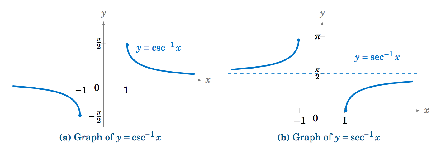
Similarly, it can be shown that the inverse cosecant $y=\csc^{-1} x$ is a function whose domain is $|x| \ge 1$ and whose range is $-\frac{\pi}{2} \le y \le \frac{\pi}{2}$, $y \ne 0$. Likewise, the inverse secant $y=\sec^{-1} x$ is a function whose domain is $|x| \ge 1$ and whose range is $0 \le y \le \pi$, $y \ne \frac{\pi}{2}$.

$$\begin{alignat}{3} \csc^{-1} (\csc\;y) ~&=~ y \quad&&\text{for \(-\frac{\pi}{2} \le y \le \frac{\pi}{2} \), \(y \ne 0\)}\label{eqn:arccsc1}\\ \csc\;(\csc^{-1} x) ~&=~ x \quad&&\text{for \(|x| \ge 1\)}\label{eqn:arccsc2} \end{alignat} \nonumber$$

$$\begin{alignat}{3} \sec^{-1} (\sec\;y) ~&=~ y \quad&&\text{for \(0 \le y \le \pi \), \(y \ne \frac{\pi}{2}\)}\label{eqn:arcsec1}\\ \sec\;(\sec^{-1} x) ~&=~ x \quad&&\text{for \(|x| \ge 1\)}\label{eqn:arcsec2} \end{alignat} \nonumber$$

It is also common to call $\cot^{-1} x$, $\csc^{-1} x$, and $\sec^{-1} x$ the arc cotangent, arc cosecant, and arc secant, respectively, of $x$. The graphs of $y=\csc^{-1} x$ and $y=\sec^{-1} x$ are shown in Figure 5.3.12:

Figure 5.3.12

Example 5.21

Prove the identity $\tan^{-1} x \;+\; \cot^{-1} x ~=~ \frac{\pi}{2}$.

Solution:

Let $\theta = \cot^{-1} x$. Using relations from Section 1.5, we have

$$\nonumber \tan\;\left( \tfrac{\pi}{2} - \theta \right) ~=~ -\tan\;\left( \theta - \tfrac{\pi}{2} \right) ~=~ \cot\;\theta ~=~ \cot\;(\cot^{-1} x) ~=~ x ~, \nonumber$$

by Equation $\ref{eqn:arccot2}$. So since $\tan\;(\tan^{-1} x) = x$ for all $x$, this means that $\tan\;(\tan^{-1} x) = \tan\;\left( \tfrac{\pi}{2} - \theta \right)$. Thus, $\tan\;(\tan^{-1} x) = \tan\;\left( \tfrac{\pi}{2} - \cot^{-1} x \right)$. Now, we know that $0 < \cot^{-1} x < \pi$, so $-\tfrac{\pi}{2} < \tfrac{\pi}{2} - \cot^{-1} x < \tfrac{\pi}{2}$, i.e. $\tfrac{\pi}{2} - \cot^{-1} x$ is in the restricted subset on which the tangent function is one-to-one. Hence, $\tan\;(\tan^{-1} x) = \tan\;\left( \tfrac{\pi}{2} - \cot^{-1} x \right)$ implies that $\tan^{-1} x = \tfrac{\pi}{2} - \cot^{-1} x$, which proves the identity.

Example 5.22

Is $\;\tan^{-1} a \;+\; \tan^{-1} b ~=~ \tan^{-1} \left( \dfrac{a+b}{1-ab} \right)\;$ an identity?

Solution

In the tangent addition Equation $\tan\;(A+B) = \dfrac{\tan\;A \;+\; \tan\;B}{1 \;-\; \tan\;A~\tan\;B}$, let $A = \tan^{-1} a$ and $B = \tan^{-1} b$. Then

$$\nonumber \begin{align*} \tan\;(\tan^{-1} a \;+\; \tan^{-1} b ) ~&=~ \dfrac{\tan\;(\tan^{-1} a) \;+\; \tan\;(\tan^{-1} b)}{1 \;-\; \tan\;(\tan^{-1} a)~\tan\;(\tan^{-1} b)}\\ \nonumber &=~ \dfrac{a+b}{1-ab}\qquad\text{by Equation \ref{eqn:arctan2}, so it seems that we have}\\ \nonumber \tan^{-1} a \;+\; \tan^{-1} b ~&=~ \tan^{-1} \left( \dfrac{a+b}{1-ab} \right) \end{align*} \nonumber$$

by definition of the inverse tangent. However, recall that $-\tfrac{\pi}{2} < \tan^{-1} x < \tfrac{\pi}{2}$ for all real numbers $x$. So in particular, we must have $-\tfrac{\pi}{2} < \tan^{-1} \left( \frac{a+b}{1-ab} \right) < \tfrac{\pi}{2}$. But it is possible that $\tan^{-1} a \;+\; \tan^{-1} b$ is not in the interval $\left(-\tfrac{\pi}{2},\tfrac{\pi}{2}\right)$. For example,

$$\tan^{-1} 1 \;+\; \tan^{-1} 2 ~=~ 1.892547 ~>~ \tfrac{\pi}{2} \approx 1.570796 ~.\nonumber$$

And we see that $\tan^{-1} \left( \frac{1+2}{1-(1)(2)} \right) = \tan^{-1} (-3) = -1.249045 \ne \tan^{-1} 1 \;+\; \tan^{-1} 2$. So the Equation is only true when $-\tfrac{\pi}{2} < \tan^{-1} a \;+\; \tan^{-1} b < \tfrac{\pi}{2}$.