8.5: Determinants and Cramer’s Rule

8.5.1 Definition and Properties of the Determinant

In this section we assign to each square matrix \(A\) a real number, called the determinant of \(A\), which will eventually lead us to yet another technique for solving consistent independent systems of linear equations. The determinant is defined recursively, that is, we define it for \(1 \times 1\) matrices and give a rule by which we can reduce determinants of \(n \times n\) matrices to a sum of determinants of \((n-1) \times (n-1)\) matrices.¹ This means we will be able to evaluate the determinant of a \(2 \times 2\) matrix as a sum of the determinants of \(1 \times 1\) matrices; the determinant of a \(3 \times 3\) matrix as a sum of the determinants of \(2 \times 2\) matrices, and so forth. To explain how we will take an \(n \times n\) matrix and distill from it an \((n-1) \times (n-1)\), we use the following notation.

Definition 8.12.

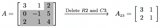
Given an \(n \times n\) matrix \(A\) where \(n>1\), the matrix \(A_{ij}\) is the \((n-1) \times (n-1)\) matrix formed by deleting the \(i\)th row of \(A\) and the \(j\)th column of \(A\).

For example, using the matrix \(A\) below, we find the matrix \(A_{23}\) by deleting the second row and third column of \(A\).

We are now in the position to define the determinant of a matrix.

Definition 8.13.

Given an \(n \times n\) matrix \(A\) the determinant of \(A\), denoted \(\det(A)\), is defined as follows

• If \(n=1\), then \(A = \left[ a_{11} \right]\) and \(\det(A) = \det\left( \left[ a_{11} \right] \right) = a_{11}\).
• If \(n>1\), then \(A = \left[ a_{ij} \right]_{n \times n}\) and \[\operatorname{det}(A)=\operatorname{det}\left(\left[a_{i j}\right]_{n \times n}\right)=a_{11} \operatorname{det}\left(A_{11}\right)-a_{12} \operatorname{det}\left(A_{12}\right)+-\ldots+(-1)^{1+n} a_{1 n} \operatorname{det}\left(A_{1 n}\right)\nonumber\]

There are two commonly used notations for the determinant of a matrix \(A\): ‘\(\det(A)\)’ and ‘\(|A|\)’ We have chosen to use the notation \(\det(A)\) as opposed to \(|A|\) because we find that the latter is often confused with absolute value, especially in the context of a \(1 \times 1\) matrix. In the expansion \(a_{11} \operatorname{det}\left(A_{11}\right)-a_{12} \operatorname{det}\left(A_{12}\right)+-\ldots+(-1)^{1+n} a_{1 n} \operatorname{det}\left(A_{1 n}\right)\), the notation ‘\(+-\ldots+(-1)^{1+n} a_{1 n}\)’ means that the signs alternate and the final sign is dictated by the sign of the quantity \((-1)^{1+n}\). Since the entries \(a_{\mbox{\tiny\)11}\), \(a_{12}\) and so forth up through \(a_{1 n}\) comprise the first row of \(A\), we say we are finding the determinant of \(A\) by ‘expanding along the first row’. Later in the section, we will develop a formula for \(\det(A)\) which allows us to find it by expanding along any row.

Applying Definition 8.13 to the matrix \(A = \left[ \begin{array}{rr} 4 & -3 \\ 2 & 1 \\ \end{array} \right]\) we get

\[\begin{array}{rcl} \det(A) & = & \det \left( \left[ \begin{array}{rr} 4 & -3 \\ 2 & 1 \\ \end{array} \right] \right)\\[13pt] & = & 4\det\left(A_11\right) - (-3)\det\left(A_12\right)\\ & = & 4 \det([1]) +3\det([2]) \\ & = & 4(1) + 3(2) \\ & = & 10 \\ \end{array}\nonumber\]

For a generic \(2 \times 2\) matrix \(A = \left[ \begin{array}{cc} a & b \\ c & d \\ \end{array} \right]\) we get

\[\begin{array}{rcl} \det(A) & = & \det \left( \left[ \begin{array}{cc} a & b \\ c & d \\ \end{array} \right] \right)\\[13pt] & = & a \det\left(A_11\right) - b \det\left(A_12\right) \\ & = & a \det\left(\left[ d \right]\right) - b \det\left(\left[c \right]\right) \\ & = & ad-bc \end{array}\nonumber\]

This formula is worth remembering

Equation 8.1.

For a \(2 \times 2\) matrix,

\[\det \left( \left[ \begin{array}{cc} a & b \\ c & d \\ \end{array} \right] \right) = ad-bc\nonumber\]

Applying Definition 8.13 to the \(3 \times 3\) matrix \(A = \left[ \begin{array}{rrr} 3 & 1 & \hphantom{-}2 \\ 0 & -1 & 5 \\ 2 & 1 & 4 \\ \end{array} \right]\) we obtain

\[\begin{array}{rcl} \det(A) & = & \det \left( \left[ \begin{array}{rrr} 3 & 1 & \hphantom{-}2 \\ 0 & -1 & 5 \\ 2 & 1 & 4 \\ \end{array} \right] \right)\\[13pt] & = & 3\det\left(A_11\right) - 1\det\left(A_12\right) + 2\det\left(A_13\right) \\[13pt] & = & 3\det \left( \left[ \begin{array}{rr} -1 & 5 \\ 1 & 4 \\ \end{array} \right] \right) - \det \left( \left[ \begin{array}{rr} 0 & 5 \\ 2 & 4 \\ \end{array} \right] \right) + 2 \det \left( \left[ \begin{array}{rr} 0 & -1 \\ 2 & 1 \\ \end{array} \right] \right) \\[13pt] & = & 3((-1)(4) - (5)(1)) - ((0)(4)-(5)(2))+2((0)(1)-(-1)(2)) \\ & = & 3(-9)-(-10)+2(2) \\ & = & -13 \\ \end{array}\nonumber\]

To evaluate the determinant of a \(4 \times 4\) matrix, we would have to evaluate the determinants of four \(3 \times 3\) matrices, each of which involves the finding the determinants of three \(2 \times 2\) matrices. As you can see, our method of evaluating determinants quickly gets out of hand and many of you may be reaching for the calculator. There is some mathematical machinery which can assist us in calculating determinants and we present that here. Before we state the theorem, we need some more terminology.

Definition 8.14.

Let \(A\) be an \(n \times n\) matrix and \(A_{ij}\) be defined as in Definition 8.12. The \(ij\) minor of \(A\), denoted \(M_{ij}\) is defined by \(M_{ij} = \det\left(A_{ij}\right)\). The \(ij\) cofactor of \(A\), denoted \(C_{ij}\) is defined by \(C_{ij} = (-1)^{i+j}M_{ij} = (-1)^{i+j}\det\left(A_{ij}\right)\).

We note that in Definition 8.13, the sum

\[a_{11} \operatorname{det}\left(A_{11}\right)-a_{12} \operatorname{det}\left(A_{12}\right)+-\ldots+(-1)^{1+n} a_{1 n} \operatorname{det}\left(A_{1 n}\right)\nonumber\]

can be rewritten as

\[a_{11}(-1)^{1+1} \operatorname{det}\left(A_{11}\right)+a_{12}(-1)^{1+2} \operatorname{det}\left(A_{12}\right)+\ldots+a_{1 n}(-1)^{1+n} \operatorname{det}\left(A_{1 n}\right)\nonumber\]

which, in the language of cofactors is

\[a_{11} C_{11}+a_{12} C_{12}+\ldots+a_{1 n} C_{1 n}\nonumber\]

We are now ready to state our main theorem concerning determinants.

Theorem 8.7.

Properties of the Determinant: Let \(A = \left[a_{ij}\right]_{n \times n}\).

• We may find the determinant by expanding along any row. That is, for any \(1 \leq k \leq n\),

  \[\operatorname{det}(A)=a_{k 1} C_{k 1}+a_{k 2} C_{k 2}+\ldots+a_{k n} C_{k n}\nonumber\]

• If \(A'\) is the matrix obtained from \(A\) by:
  • interchanging any two rows, then \(\det(A')=-\det(A)\).
  • replacing a row with a nonzero multiple (say \(c\)) of itself, then \(\det(A')=c\det(A)\)
  • replacing a row with itself plus a multiple of another row, then \(\det(A')=\det(A)\)
• If \(A\) has two identical rows, or a row consisting of all \(0\)’s, then \(\det(A) = 0\).
• If \(A\) is upper or lower triangular,^a then \(\det(A)\) is the product of the entries on the main diagonal.^b
• If \(B\) is an \(n \times n\) matrix, then \(\det(AB) = \det(A) \det(B)\).
• \(\det\left(A^{n}\right) = \det(A)^{n}\) for all natural numbers \(n\).
• \(A\) is invertible if and only if \(\det(A) \neq 0\). In this case, \(\det\left(A^{-1}\right) = \dfrac{1}{\det(A)}\).

---

^a See Exercise 8.3.1 in 8.3.

^b See page 585 in Section 8.3.

Unfortunately, while we can easily demonstrate the results in Theorem 8.7, the proofs of most of these properties are beyond the scope of this text. We could prove these properties for generic \(2 \times 2\) or even \(3 \times 3\) matrices by brute force computation, but this manner of proof belies the elegance and symmetry of the determinant. We will prove what few properties we can after we have developed some more tools such as the Principle of Mathematical Induction in Section 9.3.² For the moment, let us demonstrate some of the properties listed in Theorem 8.7 on the matrix \(A\) below. (Others will be discussed in the Exercises.)

\[A = \left[ \begin{array}{rrr} 3 & 1 & \hphantom{-}2 \\ 0 & -1 & 5 \\ 2 & 1 & 4 \\ \end{array} \right]\nonumber\]

We found \(\det(A) = -13\) by expanding along the first row. To take advantage of the \(0\) in the second row, we use Theorem 8.7 to find \(\det(A) = -13\) by expanding along that row.

\[\begin{array}{rcl} \det \left( \left[ \begin{array}{rrr} 3 & 1 & \hphantom{-}2 \\ 0 & -1 & 5 \\ 2 & 1 & 4 \\ \end{array} \right] \right)& = & 0C_21 + (-1)C_22+5C_23 \\ & = & (-1) (-1)^{2+2} \det\left(A_22\right) + 5 (-1)^{2+3}\det\left(A_23\right) \\[13pt] & = & - \det \left( \left[ \begin{array}{rr} 3 & 2 \\ 2 & 4 \\ \end{array} \right] \right) -5 \det \left( \left[ \begin{array}{rr} 3 & 1 \\ 2 & 1 \\ \end{array} \right] \right) \\[13pt] & = & -((3)(4)-(2)(2)) - 5((3)(1)-(2)(1)) \\ & = & -8-5 \\ & = & -13 \, \, \checkmark \\ \end{array}\nonumber\]

In general, the sign of \((-1)^{i+j}\) in front of the minor in the expansion of the determinant follows an alternating pattern. Below is the pattern for \(2 \times 2\), \(3 \times 3\) and \(4 \times 4\) matrices, and it extends naturally to higher dimensions.

\[\begin{array}{ccc} \left[ \begin{array}{cc} + & - \\ - & + \\ \end{array} \right] & \qquad \left[ \begin{array}{ccc} + & - & + \\ - & + & - \\ + & - & + \end{array} \right] & \qquad \left[ \begin{array}{cccc} + & - & + & - \\ - & + & - & +\\ + & - & + & - \\ - & + & - & + \end{array} \right] \end{array}\nonumber\]

The reader is cautioned, however, against reading too much into these sign patterns. In the example above, we expanded the \(3 \times 3\) matrix \(A\) by its second row and the term which corresponds to the second entry ended up being negative even though the sign attached to the minor is \((+)\). These signs represent only the signs of the \((-1)^{i+j}\) in the formula; the sign of the corresponding entry as well as the minor itself determine the ultimate sign of the term in the expansion of the determinant.

To illustrate some of the other properties in Theorem 8.7, we use row operations to transform our \(3 \times 3\) matrix \(A\) into an upper triangular matrix, keeping track of the row operations, and labeling each successive matrix.³

\[\begin{array}{ccccc} \left[ \begin{array}{rrr} 3 & 1 & \hphantom{-}2 \\ 0 & -1 & 5 \\ 2 & 1 & 4 \\ \end{array} \right] & \xrightarrow[\text{with $-\frac{2}{3}R1+R3$}]{\text{Replace $R3$}} & \left[ \begin{array}{rrr} 3 & 1 & \hphantom{-}2 \\ 0 & -1 & 5 \\ 0 & \frac{1}{3} & \frac{8}{3} \\ \end{array} \right] & \xrightarrow[\text{$\frac{1}{3}R2+R3$}]{\text{Replace $R3$ with}} & \left[ \begin{array}{rrr} 3 & 1 & 2 \\ 0 & -1 & 5 \\ 0 & 0 & \frac{13}{3} \\ \end{array} \right] \\ A & & B & & C \\ \end{array}\nonumber\]

Theorem 8.7 guarantees us that \(\det(A) = \det(B) = \det(C)\) since we are replacing a row with itself plus a multiple of another row moving from one matrix to the next. Furthermore, since \(C\) is upper triangular, \(\det(C)\) is the product of the entries on the main diagonal, in this case \(\det(C) = (3)(-1)\left(\frac{13}{3}\right) = -13\). This demonstrates the utility of using row operations to assist in calculating determinants. This also sheds some light on the connection between a determinant and invertibility. Recall from Section 8.4 that in order to find \(A^{-1}\), we attempt to transform \(A\) to \(I_{n}\) using row operations

\[\begin{array}{ccc} \left[ \begin{array}{c|c} A & I_{n} \\ \end{array} \right] & \xrightarrow{\text{Gauss Jordan Elimination}} & \left[ \begin{array}{c|c} I_{n} & A^{-1} \\ \end{array} \right] \end{array}\nonumber\]

As we apply our allowable row operations on \(A\) to put it into reduced row echelon form, the determinant of the intermediate matrices can vary from the determinant of \(A\) by at most a nonzero multiple. This means that if \(\det(A) \neq 0\), then the determinant of \(A\)’s reduced row echelon form must also be nonzero, which, according to Definition 8.4 means that all the main diagonal entries on \(A\)’s reduced row echelon form must be \(1\). That is, \(A\)’s reduced row echelon form is \(I_{n}\), and \(A\) is invertible. Conversely, if \(A\) is invertible, then \(A\) can be transformed into \(I_{n}\) using row operations. Since \(\det\left(I_{n}\right) = 1 \neq 0\), our same logic implies \(\det(A) \neq 0\). Basically, we have established that the determinant determines whether or not the matrix \(A\) is invertible.⁴

It is worth noting that when we first introduced the notion of a matrix inverse, it was in the context of solving a linear matrix equation. In effect, we were trying to ‘divide’ both sides of the matrix equation \(AX = B\) by the matrix \(A\). Just like we cannot divide a real number by \(0\), Theorem 8.7 tells us we cannot ‘divide’ by a matrix whose determinant is \(0\). We also know that if the coefficient matrix of a system of linear equations is invertible, then system is consistent and independent. It follows, then, that if the determinant of said coefficient is not zero, the system is consistent and independent.

8.5.2 Cramer’s Rule and Matrix Adjoint

In this section, we introduce a theorem which enables us to solve a system of linear equations by means of determinants only. As usual, the theorem is stated in full generality, using numbered unknowns \(x_{1}\), \(x_{2}\), etc., instead of the more familiar letters \(x\), \(y\), \(z\), etc. The proof of the general case is best left to a course in Linear Algebra.

Theorem 8.8.

Cramer’s Rule: Suppose \(AX = B\) is the matrix form of a system of \(n\) linear equations in \(n\) unknowns where \(A\) is the coefficient matrix, \(X\) is the unknowns matrix, and \(B\) is the constant matrix. If \(\det(A) \neq 0\), then the corresponding system is consistent and independent and the solution for unknowns \(x_{1}\), \(x_{2}\), …\(x_{n}\) is given by:

\[x_{j} = \dfrac{\det\left(A_{j}\right)}{\det(A)},\nonumber\]

where \(A_{j}\) is the matrix \(A\) whose \(j\)th column has been replaced by the constants in \(B\).

In words, Cramer’s Rule tells us we can solve for each unknown, one at a time, by finding the ratio of the determinant of \(A_{j}\) to that of the determinant of the coefficient matrix. The matrix \(A_{j}\) is found by replacing the column in the coefficient matrix which holds the coefficients of \(x_{j}\) with the constants of the system. The following example fleshes out this method.

Example 8.5.1

Use Cramer’s Rule to solve for the indicated unknowns.

1. Solve \(\left\{ \begin{array}{rcr} 2x_{1} - 3x_{2} & = & 4 \\ 5x_{1} + x_{2} & = & -2 \end{array} \right.\) for \(x_{1}\) and \(x_{2}\)
2. Solve \(\left\{ \begin{array}{rcr} 2x - 3y + z & = & -1 \\ x-y+z & = & 1 \\ 3x-4z & = & 0 \end{array} \right.\) for \(z\).

Solution

1. Writing this system in matrix form, we find

   \[\begin{array}{ccc} A = \left[ \begin{array}{rr} 2 & -3 \\ 5 & 1 \\ \end{array} \right] & \qquad X = \left[ \begin{array}{r} x_1 \\ x_2 \\ \end{array} \right] & \qquad B = \left[ \begin{array}{r} 4 \\ -2 \\ \end{array} \right] \\ \end{array}\nonumber\]

   To find the matrix \(A_{1}\), we remove the column of the coefficient matrix \(A\) which holds the coefficients of \(x_{1}\) and replace it with the corresponding entries in \(B\). Likewise, we replace the column of \(A\) which corresponds to the coefficients of \(x_{2}\) with the constants to form the matrix \(A_{2}\). This yields

   \[\begin{array}{cc} A_1 = \left[ \begin{array}{rr} 4 & -3 \\ -2 & 1 \\ \end{array} \right] & \qquad A_2 = \left[ \begin{array}{rr} 2 & 4 \\ 5 & -2 \\ \end{array} \right] \\ \end{array}\nonumber\]

   Computing determinants, we get \(\det(A) = 17\), \(\det\left(A_{1}\right) = -2\) and \(\det\left(A_{2}\right) = -24\), so that

   \[\begin{array}{cc} x_1 = \dfrac{\det\left(A_1\right)}{\det(A)} = -\dfrac{2}{17} & \qquad x_2 = \dfrac{\det\left(A_2\right)}{\det(A)} = -\dfrac{24}{17} \\ \end{array}\nonumber\]

   The reader can check that the solution to the system is \(\left(-\frac{2}{17}, -\frac{24}{17}\right)\).

2. To use Cramer’s Rule to find \(z\), we identify \(x_{3}\) as \(z\). We have

   \[\begin{array}{cccc} A = \left[ \begin{array}{rrr} 2 & -3 & 1 \\ 1 & -1 & 1 \\ 3 & 0 & -4 \end{array} \right] & X = \left[ \begin{array}{r} x \\ y \\ z \end{array} \right] & B = \left[ \begin{array}{r} -1 \\ 1 \\ 0 \end{array} \right] & A_3 = A_{z} = \left[ \begin{array}{rrr} 2 & -3 & -1 \\ 1 & -1 & 1 \\ 3 & 0 & 0 \end{array} \right] \\ \end{array}\nonumber\]

   Expanding both \(\det(A)\) and \(\det\left(A_{z}\right)\) along the third rows (to take advantage of the \(0\)’s) gives

   \[z = \dfrac{\det\left(A_{z}\right)}{\det(A)} = \dfrac{-12}{-10} = \dfrac{6}{5}\nonumber\]

   The reader is encouraged to solve this system for \(x\) and \(y\) similarly and check the answer.

Our last application of determinants is to develop an alternative method for finding the inverse of a matrix.⁵ Let us consider the \(3 \times 3\) matrix \(A\) which we so extensively studied in Section 8.5.1.

\[A = \left[ \begin{array}{rrr} 3 & 1 & \hphantom{-}2 \\ 0 & -1 & 5 \\ 2 & 1 & 4 \\ \end{array} \right]\nonumber\]

We found through a variety of methods that \(\det(A) = -13\). To our surprise and delight, its inverse below has a remarkable number of \(13\)’s in the denominators of its entries. This is no coincidence.

\[A^{-1} = \left[ \begin{array}{rrr} \frac{9}{13} & \frac{2}{13} & -\frac{7}{13} \\[3pt] -\frac{10}{13} & -\frac{8}{13} & \frac{15}{13} \\[3pt] -\frac{2}{13} & \frac{1}{13} & \frac{3}{13} \\ \end{array} \right]\nonumber\]

Recall that to find \(A^{-1}\), we are essentially solving the matrix equation \(AX = I_{3}\), where \(X = \left[ x_{ij} \right]_{3 \times 3}\) is a \(3 \times 3\) matrix. Because of how matrix multiplication is defined, the first column of \(I_{3}\) is the product of \(A\) with the first column of \(X\), the second column of \(I_{3}\) is the product of \(A\) with the second column of \(X\) and the third column of \(I_{3}\) is the product of \(A\) with the third column of \(X\). In other words, we are solving three equations⁶

\[\begin{array}{ccc} A\left[ \begin{array}{r} x_11 \\ x_21 \\ x_31 \end{array} \right] = \left[ \begin{array}{r} 1 \\ 0 \\ 0 \end{array} \right] & \qquad A\left[ \begin{array}{r} x_12 \\ x_22 \\ x_32 \end{array} \right] = \left[ \begin{array}{r} 0 \\ 1 \\ 0 \end{array} \right] & \qquad A\left[ \begin{array}{r} x_13 \\ x_23 \\ x_33 \end{array} \right] = \left[ \begin{array}{r} 0 \\ 0 \\ 1 \end{array} \right] \\ \end{array}\nonumber\]

We can solve each of these systems using Cramer’s Rule. Focusing on the first system, we have

\[\begin{array}{ccc} A_1 = \left[ \begin{array}{rrr} 1 & 1 & \hphantom{-}2 \\ 0 & -1 & 5 \\ 0 & 1 & 4 \\ \end{array} \right] & A_2 = \left[ \begin{array}{rrr} 3 & 1 & 2 \\ 0 & 0 & 5 \\ 2 & 0 & 4 \\ \end{array} \right] & A_3 = \left[ \begin{array}{rrr} 3 & 1 & \hphantom{-}1 \\ 0 & -1 & 0 \\ 2 & 1 & 0 \\ \end{array} \right] \end{array}\nonumber\]

If we expand \(\det\left(A_{1}\right)\) along the first row, we get

\[\begin{array}{rcl} \det\left(A_1\right) & = & \det\left( \left[ \begin{array}{rr} -1 & 5 \\ 1 & 4 \\ \end{array} \right] \right) - \det\left( \left[ \begin{array}{rr} 0 & 5 \\ 0 & 4 \\ \end{array} \right] \right) + 2 \det\left( \left[ \begin{array}{rr} 0 & -1 \\ 0 & 1 \\ \end{array} \right] \right) \\ [13pt] & = & \det\left( \left[ \begin{array}{rr} -1 & 5 \\ 1 & 4 \\ \end{array} \right] \right) \end{array}\nonumber\]

Amazingly, this is none other than the \(C_{11}\) cofactor of \(A\). The reader is invited to check this, as well as the claims that \(\det\left(A_{2}\right) = C_{12}\) and \(\det\left(A_{3}\right) = C_{13}\).⁷ (To see this, though it seems unnatural to do so, expand along the first row.) Cramer’s Rule tells us

\[\begin{array}{ccc} x_11 = \dfrac{\det\left(A_1\right)}{\det(A)} = \dfrac{C_11}{\det(A)}, & x_21 = \dfrac{\det\left(A_2\right)}{\det(A)} = \dfrac{C_12}{\det(A)}, & x_31 = \dfrac{\det\left(A_3\right)}{\det(A)} = \dfrac{C_13}{\det(A)} \end{array}\nonumber\]

So the first column of the inverse matrix \(X\) is:

\[\left[ \begin{array}{r} x_11 \\ x_21 \\ x_31 \end{array} \right] = \left[ \begin{array}{r} \dfrac{C_11}{\det(A)} \\ [13pt] \dfrac{C_12}{\det(A)} \\ [13pt] \dfrac{C_13}{\det(A)} \end{array} \right] = \dfrac{1}{\det(A)} \left[ \begin{array}{r} C_11 \\ C_12 \\ C_13 \end{array} \right]\nonumber\]

Notice the reversal of the subscripts going from the unknown to the corresponding cofactor of \(A\). This trend continues and we get \[\begin{array}{cc} \left[ \begin{array}{r} x_12 \\ x_22 \\ x_32 \end{array} \right] = \dfrac{1}{\det(A)} \left[ \begin{array}{r} C_21 \\ C_22 \\ C_23 \end{array} \right] & \qquad \left[ \begin{array}{r} x_13 \\ x_23 \\ x_33 \end{array} \right] = \dfrac{1}{\det(A)} \left[ \begin{array}{r} C_31 \\ C_32 \\ C_33 \end{array} \right] \end{array}\nonumber\]

Putting all of these together, we have obtained a new and surprising formula for \(A^{-1}\), namely

\[A^{-1} = \dfrac{1}{\det(A)} \left[ \begin{array}{ccc} C_11 & C_21 & C_31 \\ C_12 & C_22 & C_32 \\ C_13 & C_23 & C_33 \\ \end{array} \right]\nonumber\]

To see that this does indeed yield \(A^{-1}\), we find all of the cofactors of \(A\)

\[\begin{array}{rcrrcrrcr} C_11 & = & -9, & C_21 & = & -2, & C_31 & = & 7\\ C_12 & = & 10, & C_22 & = & 8, & C_32 & = & -15 \\ C_13 & = & 2, & C_23 & = & -1, & C_33 & = & -3 \\ \end{array}\nonumber\]

And, as promised,

\[A^{-1} = \dfrac{1}{\det(A)} \left[ \begin{array}{ccc} C_11 & C_21 & C_31 \\ C_12 & C_22 & C_32 \\ C_13 & C_23 & C_33 \\ \end{array} \right] = -\dfrac{1}{13} \left[ \begin{array}{rrr} -9 & -2 & 7\\ 10 & 8 & -15 \\ 2 & -1 & -3 \\ \end{array} \right] = \left[ \begin{array}{rrr} \frac{9}{13} & \frac{2}{13} & -\frac{7}{13} \\[3pt] -\frac{10}{13} & -\frac{8}{13} & \frac{15}{13} \\[3pt] -\frac{2}{13} & \frac{1}{13} & \frac{3}{13} \\ \end{array} \right]\nonumber\]

To generalize this to invertible \(n \times n\) matrices, we need another definition and a theorem. Our definition gives a special name to the cofactor matrix, and the theorem tells us how to use it along with \(\det(A)\) to find the inverse of a matrix.

Definition 8.15.

Let \(A\) be an \(n \times n\) matrix, and \(C_{ij}\) denote the \(ij\) cofactor of \(A\). The adjoint of \(A\), denoted \(\text{adj}(A)\) is the matrix whose \(ij\)-entry is the \(ji\) cofactor of \(A\), \(C_{ji}\). That is

\[\operatorname{adj}(A)=\left[\begin{array}{cccc}
C_{11} & C_{21} & \ldots & C_{n 1} \\
C_{12} & C_{22} & \ldots & C_{n 2} \\
\vdots & \vdots & & \vdots \\
C_{1 n} & C_{2 n} & \ldots & C_{n n}
\end{array}\right]\nonumber\]

This new notation greatly shortens the statement of the formula for the inverse of a matrix.

Theorem 8.9.

Let \(A\) be an invertible \(n \times n\) matrix. Then

\[A^{-1} = \dfrac{1}{\det(A)} \text{adj}(A)\nonumber\]

For \(2 \times 2\) matrices, Theorem 8.9 reduces to a fairly simple formula.

Equation 8.2.

For an invertible \(2 \times 2\) matrix,

\[\left[ \begin{array}{rr} a & b \\ c & d \\ \end{array} \right]^{-1} = \dfrac{1}{ad-bc} \left[ \begin{array}{rr} d & -b \\ -c & a \\ \end{array} \right]\nonumber\]

The proof of Theorem 8.9 is, like so many of the results in this section, best left to a course in Linear Algebra. In such a course, not only do you gain some more sophisticated proof techniques, you also gain a larger perspective. The authors assure you that persistence pays off. If you stick around a few semesters and take a course in Linear Algebra, you’ll see just how pretty all things matrix really are - in spite of the tedious notation and sea of subscripts. Within the scope of this text, we will prove a few results involving determinants in Section 9.3 once we have the Principle of Mathematical Induction well in hand. Until then, make sure you have a handle on the mechanics of matrices and the theory will come eventually.

8.5.3. Exercises

In Exercises 1 - 8, compute the determinant of the given matrix. (Some of these matrices appeared in Exercises 1 - 8 in Section 8.4.)

1. \(B = \left[ \begin{array}{rr} 12 & -7 \\ -5 & 3 \end{array} \right]\)
2. \(C = \left[ \begin{array}{rr} 6 & 15 \\ 14 & 35 \end{array} \right]\)
3. \(Q = \left[ \begin{array}{rr} x & x^{2} \\ 1 & 2x \end{array} \right] \vphantom{ \left[ \begin{array}{rr} \dfrac{1}{x^{3}} & \dfrac{\ln(x)}{x^{3}} \\[10pt] -\dfrac{3}{x^{4}} & \dfrac{1 - 3\ln(x)}{x^{4}} \end{array} \right]}\)
4. \(L = \left[ \begin{array}{rr} \dfrac{1}{x^{3}} & \dfrac{\ln(x)}{x^{3}} \\[10pt] -\dfrac{3}{x^{4}} & \dfrac{1 - 3\ln(x)}{x^{4}} \end{array} \right]\)
5. \(F = \left[ \begin{array}{rrr} 4 & \hphantom{-}6 & -3 \\ 3 & 4 & -3 \\ 1 & 2 & 6 \end{array} \right]\)
6. \(G = \left[ \begin{array}{rrr} 1 & \hphantom{1}2 & 3 \\ 2 & 3 & 11 \\ 3 & 4 & 19 \end{array} \right]\)
7. \(V = \left[ \begin{array}{rrr} i & j & k \\ -1 & 0 & 5 \\ 9 & -4 & -2 \end{array} \right] \vphantom{\left[ \begin{array}{rrrr} 1 & 0 & -3 & 0 \\ 2 & -2 & 8 & 7 \\ -5 & 0 & 16 & 0 \\ 1 & 0 & 4 & 1 \end{array} \right]}\)
8. \(H = \left[ \begin{array}{rrrr} 1 & 0 & -3 & 0 \\ 2 & -2 & 8 & 7 \\ -5 & 0 & 16 & 0 \\ 1 & 0 & 4 & 1 \end{array} \right]\)

In Exercises 9 - 14, use Cramer’s Rule to solve the system of linear equations.

9. \(\left\{ \begin{array}{rcr} 3x + 7y & = & 26 \\ 5x + 12y & = & 39 \end{array} \right.\)
10. \(\left\{ \begin{array}{rcr} 2x-4y & = & 5 \\ 10x + 13y & = & -6 \end{array} \right.\)
11. \(\left\{ \begin{array}{rcr} x + y & = & 8000 \\ 0.03x + 0.05y & = & 250 \end{array} \right.\)
12. \(\left\{ \begin{array}{rcr} \frac{1}{2}x - \frac{1}{5}y & = & 1 \\ 6x +7y & = & 3 \end{array} \right.\)
13. \(\left\{ \begin{array}{rcr} x + y + z & = & 3 \\ 2x - y + z & = & 0 \\ -3x + 5y + 7z & = & 7 \end{array} \right.\)
14. \(\left\{ \begin{array}{rcr} 3x + y - 2z & = & 10 \\ 4x - y + z & = & 5 \\ x -3y - 4z & = & -1 \end{array} \right.\)

In Exercises 15 - 16, use Cramer’s Rule to solve for \(x_{4}\).

15. \(\left\{ \begin{array}{rcr} x_{1} - x_{3} & = & -2 \\ 2x_{2} - x_{4} & = & 0 \\ x_{1} - 2x_{2} + x_{3} & = & 0 \\ -x_{3} + x_{4} & = & 1 \end{array} \right.\)
16. \(\left\{ \begin{array}{rcr} 4x_{1} + x_{2} & = & 4 \\ x_{2} - 3x_{3} & = & 1 \\ 10x_{1} +x_{3} + x_{4} & = & 0 \\ -x_{2} + x_{3} & = & -3 \end{array} \right.\)

In Exercises 17 - 18, find the inverse of the given matrix using their determinants and adjoints.

17. \(B = \left[ \begin{array}{rr} 12 & -7 \\ -5 & 3 \end{array} \right] \vphantom{\left[ \begin{array}{rrr} 4 & \hphantom{-}6 & -3 \\ 3 & 4 & -3 \\ 1 & 2 & 6 \end{array} \right]}\) [invadjfirst]
18. \(F = \left[ \begin{array}{rrr} 4 & \hphantom{-}6 & -3 \\ 3 & 4 & -3 \\ 1 & 2 & 6 \end{array} \right]\)
19. Carl’s Sasquatch Attack! Game Card Collection is a mixture of common and rare cards. Each common card is worth \(\$0.25\) while each rare card is worth \(\$0.75\). If his entire 117 card collection is worth \(\$48.75\), how many of each kind of card does he own?
20. How much of a 5 gallon \(40\%\) salt solution should be replaced with pure water to obtain 5 gallons of a \(15 \%\) solution?
21. How much of a 10 liter \(30\%\) acid solution must be replaced with pure acid to obtain 10 liters of a \(50\%\) solution?
22. Daniel’s Exotic Animal Rescue houses snakes, tarantulas and scorpions. When asked how many animals of each kind he boards, Daniel answered: ‘We board 49 total animals, and I am responsible for each of their 272 legs and 28 tails.’ How many of each animal does the Rescue board? (Recall: tarantulas have 8 legs and no tails, scorpions have 8 legs and one tail, and snakes have no legs and one tail.)
23. This exercise is a continuation of Exercise 16 in Section 8.4. Just because a system is consistent independent doesn’t mean it will admit a solution that makes sense in an applied setting. Using the nutrient values given for Ippizuti Fish, Misty Mushrooms, and Sun Berries, use Cramer’s Rule to determine the number of servings of Ippizuti Fish needed to meet the needs of a daily diet which requires 2500 calories, 1000 grams of protein, and 400 milligrams of Vitamin X. Now use Cramer’s Rule to find the number of servings of Misty Mushrooms required. Does a solution to this diet problem exist?
24. Let \(R = \left[ \begin{array}{rr} -7 & 3 \\ 11 & \hphantom{-} 2 \end{array} \right], \;\;\; S = \left[ \begin{array}{rr} 1 & -5 \\ 6 & 9 \end{array} \right] \;\;\; T = \left[ \begin{array}{rr} 11 & \hphantom{-} 2 \\ -7 & 3 \end{array} \right], \mbox{ and } U = \left[ \begin{array}{rr} -3 & 15 \\ 6 & 9 \end{array} \right]\)
    1. Show that \(\det(RS) = \det(R)\det(S)\)
    2. Show that \(\det(T) = -\det(R)\)
    3. Show that \(\det(U) = -3\det(S)\)
25. For \(M\), \(N\), and \(P\) below, show that \(\det(M) = 0\), \(\det(N) = 0\) and \(\det(P) = 0\). \[M = \left[ \begin{array}{rrr} 1 & 2 & 3 \\ 0 & 0 & 0 \\ 7 & 8 & 9 \end{array} \right], \quad N = \left[ \begin{array}{rrr} 1 & 2 & 3 \\ 1 & 2 & 3 \\ 4 & 5 & 6 \end{array} \right] , \quad P = \left[ \begin{array}{rrr} 1 & 2 & 3 \\ -2 & -4 & -6 \\ 7 & 8 & 9 \end{array} \right]\nonumber\]
26. Let \(A\) be an arbitrary invertible \(3 \times 3\) matrix.
    1. Show that \(\det(I_{3}) = 1\). (See footnote⁸ below.)
    2. Using the facts that \(AA^{-1} = I_{3}\) and \(\det(AA^{-1}) = \det(A)\det(A^{-1})\), show that \[\det(A^{-1}) = \dfrac{1}{\det(A)}\nonumber\]

The purpose of Exercises 27 - 30 is to introduce you to the eigenvalues and eigenvectors of a matrix.⁹ We begin with an example using a \(2 \times 2\) matrix and then guide you through some exercises using a \(3 \times 3\) matrix. Consider the matrix \[C = \left[ \begin{array}{rr} 6 & 15 \\ 14 & 35 \end{array} \right]\nonumber\] from Exercise 2. We know that \(\det(C) = 0\) which means that \(CX = 0_{2 \times 2}\) does not have a unique solution. So there is a nonzero matrix \(Y\) with \(CY = 0_{2 \times 2}\). In fact, every matrix of the form \[Y = \left[ \begin{array}{r} -\frac{5}{2}t \\[3pt] t \end{array} \right]\nonumber\] is a solution to \(CX = 0_{2 \times 2}\), so there are infinitely many matrices such that \(CX = 0_{2 \times 2}\). But consider the matrix \[X_41 = \left[ \begin{array}{r} 3 \\ 7 \end{array} \right]\nonumber\] It is NOT a solution to \(CX = 0_{2 \times 2}\), but rather, \[CX_41= \left[ \begin{array}{rr} 6 & 15 \\ 14 & 35 \end{array} \right] \left[ \begin{array}{r} 3 \\ 7 \end{array} \right] = \left[ \begin{array}{r} 123 \\ 287 \end{array} \right] = 41\left[ \begin{array}{r} 3 \\ 7 \end{array} \right]\nonumber\] In fact, if \(Z\) is of the form \[Z = \left[ \begin{array}{r} \frac{3}{7}t \\[3pt] t \end{array} \right]\nonumber\] then \[CZ = \left[ \begin{array}{rr} 6 & 15 \\ 14 & 35 \end{array} \right] \left[ \begin{array}{r} \frac{3}{7}t \\[3pt] t \end{array} \right] = \left[ \begin{array}{r} \frac{123}{7}t \\[3pt] 41t \end{array} \right] = 41\left[ \begin{array}{r} \frac{3}{7}t \\[3pt] t \end{array} \right] = 41Z\nonumber\] for all \(t\). The big question is “How did we know to use \(41\)?”

We need a number \(\lambda\) such that \(CX = \lambda X\) has nonzero solutions. We have demonstrated that \(\lambda = 0\) and \(\lambda = 41\) both worked. Are there others? If we look at the matrix equation more closely, what we really wanted was a nonzero solution to \((C - \lambda I_{2})X = 0_{2 \times 2}\) which we know exists if and only if the determinant of \(C - \lambda I_{2}\) is zero.¹⁰ So we computed \[\det(C - \lambda I_2) = \det\left(\left[ \begin{array}{rr} 6 - \lambda & 15 \\ 14 & 35 - \lambda \end{array} \right] \right) = (6 - \lambda)(35 - \lambda) - 14 \cdot 15 = \lambda^{2} - 41 \lambda\nonumber\] This is called the characteristic polynomial of the matrix \(C\) and it has two zeros: \(\lambda = 0\) and \(\lambda = 41\). That’s how we knew to use \(41\) in our work above. The fact that \(\lambda = 0\) showed up as one of the zeros of the characteristic polynomial just means that \(C\) itself had determinant zero which we already knew. Those two numbers are called the eigenvalues of \(C\). The corresponding matrix solutions to \(CX = \lambda X\) are called the eigenvectors of \(C\) and the ‘vector’ portion of the name will make more sense after you’ve studied vectors.

Now it’s your turn. In the following exercises, you’ll be using the matrix \(G\) from Exercise 6.\[G = \left[ \begin{array}{rrr} 1 & \hphantom{1}2 & 3 \\ 2 & 3 & 11 \\ 3 & 4 & 19 \end{array} \right]\nonumber\]

27. Show that the characteristic polynomial of \(G\) is \(p(\lambda) = -\lambda(\lambda - 1)(\lambda - 22)\). That is, compute \(\text{det}\left(G - \lambda I_{3}\right)\).
28. Let \(G_0 = G\). Find the parametric description of the solution to the system of linear equations given by \(GX = 0_{3 \times 3}\).
29. Let \(G_{1} = G - I_{3}\). Find the parametric description of the solution to the system of linear equations given by \(G_{1}X = 0_{3 \times 3}\). Show that any solution to \(G_{1}X = 0_{3 \times 3}\) also has the property that \(GX = 1X\).
30. Let \(G_{22} = G - 22 I_{3}\). Find the parametric description of the solution to the system of linear equations given by \(G_{22}X = 0_{3 \times 3}\). Show that any solution to \(G_{22}X = 0_{3 \times 3}\) also has the property that \(GX = 22X\).

Answers

1. \(\det(B) = 1\)
2. \(\det(C) = 0\)
3. \(\det(Q) = x^{2} \phantom{\dfrac{1}{x^{7}}}\)
4. \(\det(L) = \dfrac{1}{x^{7}}\)
5. \(\det(F) = -12\)
6. \(\det(G) = 0\)
7. \(\det(V) = 20i + 43j + 4k\)
8. \(\det(H) = -2\)
9. \(x = 39, \; y = -13\)
10. \(x = \frac{41}{66}, \; y=-\frac{31}{33}\)
11. \(x=7500, \; y=500\)
12. \(x = \frac{76}{47}, \; y=-\frac{45}{47}\)
13. \(x = 1, \; y = 2, \; z = 0\)
14. \(x = \frac{121}{60}, \; y = \frac{131}{60}, \; z = -\frac{53}{60}\)
15. \(x_{4} = 4\)
16. \(x_{4} = -1\)
17. \(B^{-1} = \left[ \begin{array}{rr} 3 & 7 \\ 5 & 12 \end{array} \right]\)
18. \(F^{-1} = \left[ \begin{array}{rrr} -\frac{5}{2} & \frac{7}{2} & \frac{1}{2} \\[3pt] \frac{7}{4} & -\frac{9}{4} & -\frac{1}{4} \\[3pt] -\frac{1}{6} & \frac{1}{6} & \frac{1}{6} \end{array} \right]\)
19. Carl owns 78 common cards and 39 rare cards.
20. \(3.125\) gallons.
21. \(\frac{20}{7} \approx 2.85\) liters.
22. The rescue houses 15 snakes, 21 tarantulas and 13 scorpions.
23. Using Cramer’s Rule, we find we need 53 servings of Ippizuti Fish to satisfy the dietary requirements. The number of servings of Misty Mushrooms required, however, is \(-1120\). Since it’s impossible to have a negative number of servings, there is no solution to the applied problem, despite there being a solution to the mathematical problem. A cautionary tale about using Cramer’s Rule: just because you are guaranteed a mathematical answer for each variable doesn’t mean the solution will make sense in the ‘real’ world.

---

Reference

¹ We will talk more about the term ‘recursively’ in Section 9.1.

² For a very elegant treatment, take a course in Linear Algebra. There, you will most likely see the treatment of determinants logically reversed than what is presented here. Specifically, the determinant is defined as a function which takes a square matrix to a real number and satisfies some of the properties in Theorem 8.7. From that function, a formula for the determinant is developed.

³ Essentially, we follow the Gauss Jordan algorithm but we don’t care about getting leading 1’s.

⁴ In Section 8.5.2, we learn determinants (specifically cofactors) are deeply connected with the inverse of a matrix.

⁵ We are developing a method in the forthcoming discussion. As with the discussion in Section 8.4 when we developed the first algorithm to find matrix inverses, we ask that you indulge us.

⁶ The reader is encouraged to stop and think this through.

⁷ In a solid Linear Algebra course you will learn that the properties in Theorem 8.7 hold equally well if the word ‘row’ is replaced by the word ‘column’. We’re not going to get into column operations in this text, but they do make some of what we’re trying to say easier to follow.

⁸ If you think about it for just a moment, you’ll see that det \(\left(I_{n}\right)=1\) for any natural number \(n\). The formal proof of this fact requires the Principle of Mathematical Induction (Section 9.3) so we’ll stick with \(n = 3\) for the time being.

⁹ This material is usually given its own chapter in a Linear Algebra book so clearly we’re not able to tell you everything you need to know about eigenvalues and eigenvectors. They are a nice application of determinants, though, so we’re going to give you enough background so that you can start playing around with them.

¹⁰ Think about this.