5.2: Transformation of Graphs
- Page ID
- 48976

\( \newcommand{\vecs}[1]{\overset { \scriptstyle \rightharpoonup} {\mathbf{#1}} } \)
\( \newcommand{\vecd}[1]{\overset{-\!-\!\rightharpoonup}{\vphantom{a}\smash {#1}}} \)
\( \newcommand{\dsum}{\displaystyle\sum\limits} \)
\( \newcommand{\dint}{\displaystyle\int\limits} \)
\( \newcommand{\dlim}{\displaystyle\lim\limits} \)
\( \newcommand{\id}{\mathrm{id}}\) \( \newcommand{\Span}{\mathrm{span}}\)
( \newcommand{\kernel}{\mathrm{null}\,}\) \( \newcommand{\range}{\mathrm{range}\,}\)
\( \newcommand{\RealPart}{\mathrm{Re}}\) \( \newcommand{\ImaginaryPart}{\mathrm{Im}}\)
\( \newcommand{\Argument}{\mathrm{Arg}}\) \( \newcommand{\norm}[1]{\| #1 \|}\)
\( \newcommand{\inner}[2]{\langle #1, #2 \rangle}\)
\( \newcommand{\Span}{\mathrm{span}}\)
\( \newcommand{\id}{\mathrm{id}}\)
\( \newcommand{\Span}{\mathrm{span}}\)
\( \newcommand{\kernel}{\mathrm{null}\,}\)
\( \newcommand{\range}{\mathrm{range}\,}\)
\( \newcommand{\RealPart}{\mathrm{Re}}\)
\( \newcommand{\ImaginaryPart}{\mathrm{Im}}\)
\( \newcommand{\Argument}{\mathrm{Arg}}\)
\( \newcommand{\norm}[1]{\| #1 \|}\)
\( \newcommand{\inner}[2]{\langle #1, #2 \rangle}\)
\( \newcommand{\Span}{\mathrm{span}}\) \( \newcommand{\AA}{\unicode[.8,0]{x212B}}\)
\( \newcommand{\vectorA}[1]{\vec{#1}} % arrow\)
\( \newcommand{\vectorAt}[1]{\vec{\text{#1}}} % arrow\)
\( \newcommand{\vectorB}[1]{\overset { \scriptstyle \rightharpoonup} {\mathbf{#1}} } \)
\( \newcommand{\vectorC}[1]{\textbf{#1}} \)
\( \newcommand{\vectorD}[1]{\overrightarrow{#1}} \)
\( \newcommand{\vectorDt}[1]{\overrightarrow{\text{#1}}} \)
\( \newcommand{\vectE}[1]{\overset{-\!-\!\rightharpoonup}{\vphantom{a}\smash{\mathbf {#1}}}} \)
\( \newcommand{\vecs}[1]{\overset { \scriptstyle \rightharpoonup} {\mathbf{#1}} } \)
\(\newcommand{\longvect}{\overrightarrow}\)
\( \newcommand{\vecd}[1]{\overset{-\!-\!\rightharpoonup}{\vphantom{a}\smash {#1}}} \)
\(\newcommand{\avec}{\mathbf a}\) \(\newcommand{\bvec}{\mathbf b}\) \(\newcommand{\cvec}{\mathbf c}\) \(\newcommand{\dvec}{\mathbf d}\) \(\newcommand{\dtil}{\widetilde{\mathbf d}}\) \(\newcommand{\evec}{\mathbf e}\) \(\newcommand{\fvec}{\mathbf f}\) \(\newcommand{\nvec}{\mathbf n}\) \(\newcommand{\pvec}{\mathbf p}\) \(\newcommand{\qvec}{\mathbf q}\) \(\newcommand{\svec}{\mathbf s}\) \(\newcommand{\tvec}{\mathbf t}\) \(\newcommand{\uvec}{\mathbf u}\) \(\newcommand{\vvec}{\mathbf v}\) \(\newcommand{\wvec}{\mathbf w}\) \(\newcommand{\xvec}{\mathbf x}\) \(\newcommand{\yvec}{\mathbf y}\) \(\newcommand{\zvec}{\mathbf z}\) \(\newcommand{\rvec}{\mathbf r}\) \(\newcommand{\mvec}{\mathbf m}\) \(\newcommand{\zerovec}{\mathbf 0}\) \(\newcommand{\onevec}{\mathbf 1}\) \(\newcommand{\real}{\mathbb R}\) \(\newcommand{\twovec}[2]{\left[\begin{array}{r}#1 \\ #2 \end{array}\right]}\) \(\newcommand{\ctwovec}[2]{\left[\begin{array}{c}#1 \\ #2 \end{array}\right]}\) \(\newcommand{\threevec}[3]{\left[\begin{array}{r}#1 \\ #2 \\ #3 \end{array}\right]}\) \(\newcommand{\cthreevec}[3]{\left[\begin{array}{c}#1 \\ #2 \\ #3 \end{array}\right]}\) \(\newcommand{\fourvec}[4]{\left[\begin{array}{r}#1 \\ #2 \\ #3 \\ #4 \end{array}\right]}\) \(\newcommand{\cfourvec}[4]{\left[\begin{array}{c}#1 \\ #2 \\ #3 \\ #4 \end{array}\right]}\) \(\newcommand{\fivevec}[5]{\left[\begin{array}{r}#1 \\ #2 \\ #3 \\ #4 \\ #5 \\ \end{array}\right]}\) \(\newcommand{\cfivevec}[5]{\left[\begin{array}{c}#1 \\ #2 \\ #3 \\ #4 \\ #5 \\ \end{array}\right]}\) \(\newcommand{\mattwo}[4]{\left[\begin{array}{rr}#1 \amp #2 \\ #3 \amp #4 \\ \end{array}\right]}\) \(\newcommand{\laspan}[1]{\text{Span}\{#1\}}\) \(\newcommand{\bcal}{\cal B}\) \(\newcommand{\ccal}{\cal C}\) \(\newcommand{\scal}{\cal S}\) \(\newcommand{\wcal}{\cal W}\) \(\newcommand{\ecal}{\cal E}\) \(\newcommand{\coords}[2]{\left\{#1\right\}_{#2}}\) \(\newcommand{\gray}[1]{\color{gray}{#1}}\) \(\newcommand{\lgray}[1]{\color{lightgray}{#1}}\) \(\newcommand{\rank}{\operatorname{rank}}\) \(\newcommand{\row}{\text{Row}}\) \(\newcommand{\col}{\text{Col}}\) \(\renewcommand{\row}{\text{Row}}\) \(\newcommand{\nul}{\text{Nul}}\) \(\newcommand{\var}{\text{Var}}\) \(\newcommand{\corr}{\text{corr}}\) \(\newcommand{\len}[1]{\left|#1\right|}\) \(\newcommand{\bbar}{\overline{\bvec}}\) \(\newcommand{\bhat}{\widehat{\bvec}}\) \(\newcommand{\bperp}{\bvec^\perp}\) \(\newcommand{\xhat}{\widehat{\xvec}}\) \(\newcommand{\vhat}{\widehat{\vvec}}\) \(\newcommand{\uhat}{\widehat{\uvec}}\) \(\newcommand{\what}{\widehat{\wvec}}\) \(\newcommand{\Sighat}{\widehat{\Sigma}}\) \(\newcommand{\lt}{<}\) \(\newcommand{\gt}{>}\) \(\newcommand{\amp}{&}\) \(\definecolor{fillinmathshade}{gray}{0.9}\)For a given function, we now study how the graph of the function changes when performing elementary operations, such as adding, subtracting, or multiplying a constant number to the input or output. We will study the behavior in five specific examples.
- Consider the following graphs:
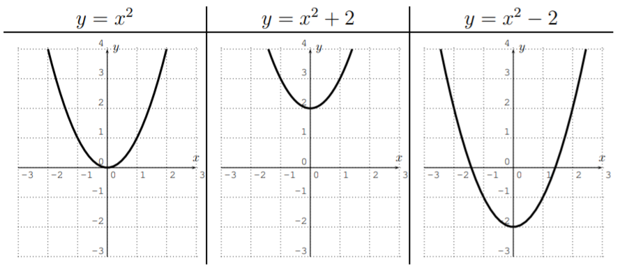
We see that the function \(y=x^2\) is shifted up by \(2\) units, respectively down by \(2\) units. In general, we have:
Consider the graph of a function \(y=f(x)\). Then, the graph of \(y=f(x)+c\) is that of \(y=f(x)\) shifted up or down by \(c\). If \(c\) is positive, the graph is shifted up, if \(c\) is negative, the graph is shifted down.
- Next, we consider the transformation of \(y=x^2\) given by adding or subtracting a constant to the input \(x\).
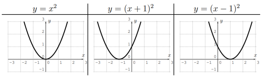
Now, we see that the function is shifted to the left or right. Note, that \(y=(x+1)^2\) shifts the function to the left, which can be seen to be correct, since the input \(x=-1\) gives the output \(y=((-1)+1)^2=0^2=0\).
Consider the graph of a function \(y=f(x)\). Then, the graph of \(y=f(x+c)\) is that of \(y=f(x)\) shifted to the left or right by \(c\). If \(c\) is positive, the graph is shifted to the left, if \(c\) is negative, the graph is shifted to the right.
- Another transformation is given by multiplying the function by a fixed positive factor.
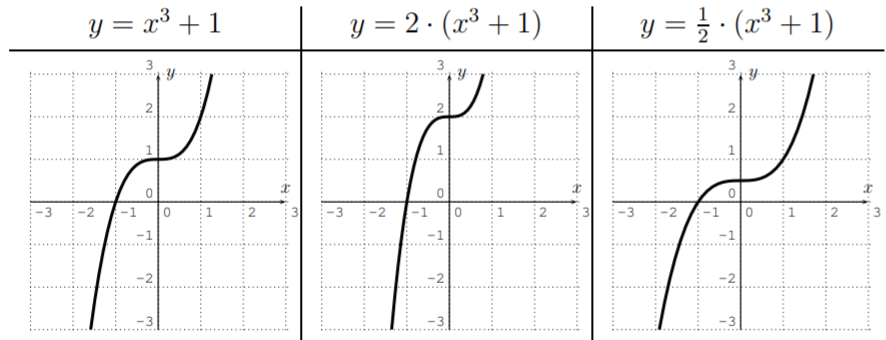
This time, the function is stretched away or compressed towards the \(x\)-axis.
Consider the graph of a function \(y=f(x)\) and let \(c>0\). Then, the graph of \(y=c\cdot f(x)\) is that of \(y=f(x)\) stretched away or compressed towards the \(x\)-axis by a factor \(c\). If \(c>1\), the graph is stretched away from the \(x\)-axis, if \(0<c<1\), the graph is compressed towards the \(x\)-axis.
- Similarly, we can multiply the input by a positive factor.
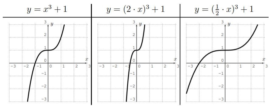
This time, the function is stretched away or compressed towards the \(y\)-axis.
Consider the graph of a function \(y=f(x)\) and let \(c>0\). Then, the graph of \(y=f(c\cdot x)\) is that of \(y=f(x)\) stretched away or compressed towards the \(y\)-axis by a factor \(c\). If \(c>1\), the graph is compressed towards the \(y\)-axis, if \(0<c<1\), the graph is stretched away from the \(y\)-axis.
- The last transformation is given by multiplying \((-1)\) to the input or output, as displayed in the following chart.
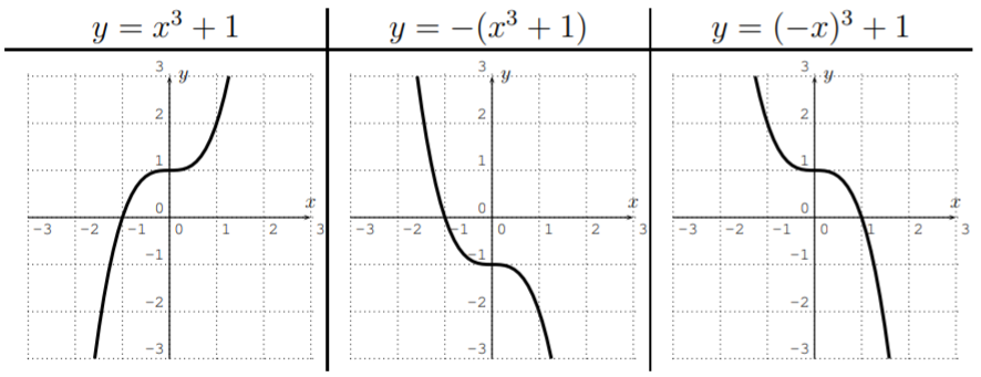
Here, the function is reflected either about the \(x\)-axis or the \(y\)-axis.
Consider the graph of a function \(y=f(x)\). Then, the graph of \(y=-f(x)\) is that of \(y=f(x)\) reflected about the \(x\)-axis. Furthermore, the graph of \(y=f(-x)\) is that of \(y=f(x)\) reflected about the \(y\)-axis.
Guess the formula for the function, based on the basic graphs in Section 5.1 and the transformations described above.
Solution
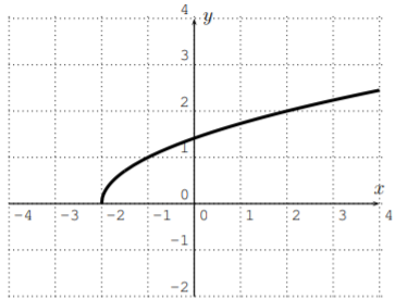
- This is the square-root function shifted to the left by \(2\). Thus, by Observation, this is the function \(f(x)=\sqrt{x+2}\).
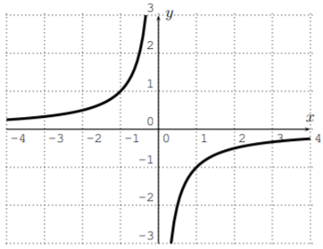
- This is the graph of \(y=\dfrac 1 x\) reflected about the \(x\)-axis (or also \(y=\dfrac 1 x\) reflected about the \(y\)-axis). In either case, we obtain the rule \(y=-\dfrac 1 x\).
-
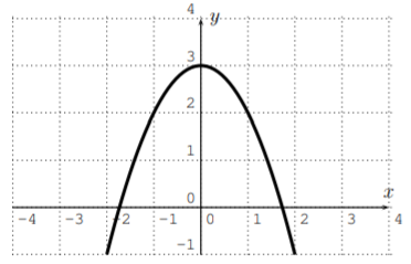
This is a parabola reflected about the \(x\)-axis and then shifted up by \(3\). Thus, we get: \[\begin{aligned}
&y=x^{2} \\
\text{reflecting about the x-axis gives }&y=-x^{2} \\
\text{shifting the graph up by 3 gives }&y=-x^{2}+3
\end{aligned} \nonumber \] -
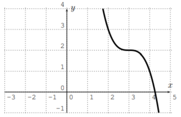
Starting from the graph of the cubic equation \(y=x^3\), we need to reflect about the \(x\)-axis (or also \(y\)-axis), then shift up by \(2\) and to the right by \(3\). These transformations affect the formula as follows: \[\begin{aligned}
& y=x^{3} \\
\text {reflecting about the x-axis gives } & y=-x^{3}\\
\text{shifting up by 2 gives } & y=-x^{3}+2\\
\text{shifting the the right by 3 gives } & y=-(x-3)^{3}+2
\end{aligned} \nonumber \]
All these answers can be checked by graphing the function with the TI-84.
Sketch the graph of the function, based on the basic graphs in Section 5.1 and the transformations described above.
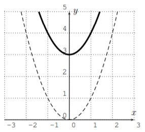
- \(y=x^2+3\)
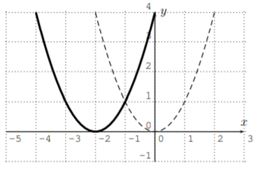
- \(y=(x+2)^2\)
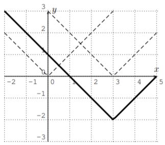
- \(y=|x-3|-2\)
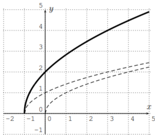
- \(y=2\cdot \sqrt{x+1}\)
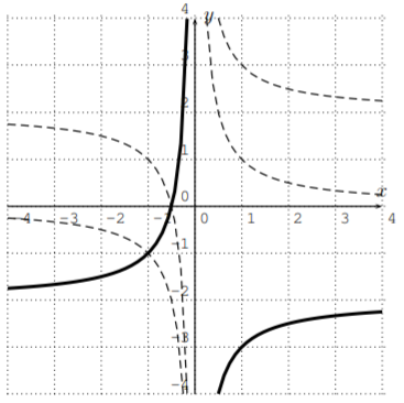
- \(y=-\left(\dfrac 1 {x}+2\right)\)
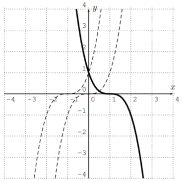
- \(y=(-x+1)^3\)
Solution
- This is the parabola \(y=x^2\) shifted up by \(3\). The graph is shown below.
- \(y=(x+2)^2\) is the parabola \(y=x^2\) shifted \(2\) units to the left.
- The graph of the function \(f(x)=|x-3|-2\) is the absolute value shifted to the right by \(3\) and down by \(2\). (Alternatively, we can first shift down by \(2\) and then to the right by \(3\).)
- Similarly, to get from the graph of \(y=\sqrt{x}\) to the graph of \(y=\sqrt{x+1}\), we shift the graph to the left, and then for \(y=2\cdot \sqrt{x+1}\), we need to stretch the graph by a factor \(2\) away from the \(x\)-axis. (Alternatively, we could first stretch the the graph away from the \(x\)-axis, then shift the graph by \(1\) to the left.)
- For \(y=-\left(\dfrac 1 x +2\right)\), we start with \(y=\dfrac 1 x\) and add \(2\), giving \(y=\dfrac 1 x +2\), which shifts the graph up by \(2\). Then, taking the negative gives \(y=-\left(\dfrac 1 x +2\right)\), which corresponds to reflecting the graph about the \(x\)-axis. Note, that in this case, we cannot perform these transformations in the opposite order, since the negative of \(y=\dfrac 1 x\) gives \(y=-\dfrac 1 x\), and adding \(2\) gives \(y=-\dfrac 1 x+2\) which is not equal to \(-(\dfrac 1 x+2)\).
- We start with \(y=x^3\). Adding \(1\) in the argument, \(y=(x+1)^3\), shifts its graph to the left by \(1\). Then, taking the negative in the argument gives \(y=(-x+1)^3\), which reflects the graph about the \(y\)-axis. Here, the order in which we perform these transformations is again important. In fact, if we first take the negative in the argument, we obtain \(y=(-x)^3\). Then, adding one in the argument would give \(y=(-(x+1))^3=(-x-1)^3\) which is different than our given function \(y=(-x+1)^3\).
All these solutions may also easily be checked by using the graphing function of the calculator.
- The graph of \(f(x)=|x^3-5|\) is stretched away from the \(y\)-axis by a factor of \(3\). What is the formula for the new function?
- The graph of \(f(x)=\sqrt{6x^2+3}\) is shifted up \(5\) units, and then reflected about the \(x\)-axis. What is the formula for the new function?
- How are the graphs of \(y=2x^3+5x-9\) and \(y=2(x-2)^3+5(x-2)-9\) related?
- How are the graphs of \(y=(x-2)^2\) and \(y=(-x+3)^2\) related?
Solution
- By Observation on page , we have to multiply the argument by \(\frac 1 3\). The new function is therefore:
\[f\Big(\dfrac 1 3 \cdot x\Big)=\left|\Big(\dfrac 1 3\cdot x \Big)^3-5\right|=\left|\dfrac 1 {27} \cdot x^3-5\right| \nonumber\]
- After the shift, we have the graph of a new function \(y=\sqrt{6x^2+3}+5\).Then, a reflection about the \(x\)-axis gives the graph of the function \(y=-(\sqrt{6x^2+3}+5)\).
- By Observation on page , we see that we need to shift the graph of \(y=2x^3+5x-9\) by \(2\) units to the right.
-
The formulas can be transformed into each other as follows: \[\begin{align*}
\text{We begin with } & y=(x-2)^{2}\\
\text{Replacing x by x+5 gives } & y=((x+5)-2)^{2}=(x+3)^{2}\\
\text{Replacing x by -x gives } & y=((-x)+3)^{2}=(-x+3)^{2}
\end{align*} \nonumber \]Therefore, we have performed a shift to the left by \(5\), and then a reflection about the \(y\)-axis.We want to point out that there is a second solution for this problem: We begin with & \(y=(x-2)^2\).
Replacing \(x\) by \(-x\) gives \(y=((-x)-2)^2=(-x-2)^2\).
Replacing \(x\) by \(x-5\) gives \(y=(-(x-5)-2)^2=(-x+5-2)^2=(-x+3)^2\). Therefore, we could also first perform a reflection about the \(y\)-axis, and then shift the graph to the right by \(5\).
Some of the above functions have special symmetries, which we investigate now.
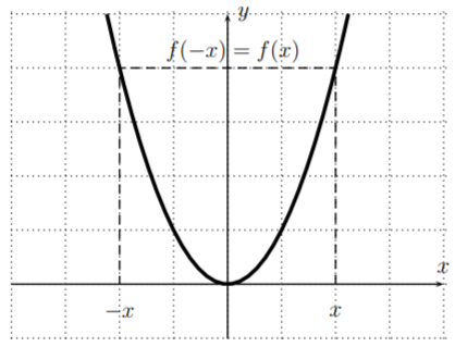
A function \(f\) is called even if \(f(-x)=f(x)\) for all \(x\).
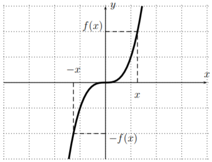
Similarly, a function \(f\) is called odd if \(f(-x)=-f(x)\) for all \(x\).
Determine, if the following functions are even, odd, or neither. \(f(x)=x^2\), \(g(x)=x^3\), & \(h(x)=x^4\), \(k(x)=x^5\),
\(l(x)=4x^5+7x^3-2x\), & \(m(x)=x^2+5x\).
Solution
The function \(f(x)=x^2\) is even, since \(f(-x)=(-x)^2=x^2\). Similarly, \(g(x)=x^3\) is odd, \(h(x)=x^4\) is even, and \(k(x)=x^5\) is odd, since
\[\begin{aligned} g(-x)&=(-x)^3=-x^3=-g(x) \\ h(-x)&=(-x)^4=x^4=h(x) \\ k(-x)&=(-x)^5=-x^5=-k(x) \end{aligned}\]
Indeed, we see that a function \(y=x^n\) is even, precisely when \(n\) is even, and \(y=x^n\) is odd, precisely when \(n\) is odd. (These examples are in fact the motivation behind defining even and odd functions as in Definition Even-Odd above.)
Next, in order to determine if the function \(l\) is even or odd, we calculate \(l(-x)\) and compare it with \(l(x)\).
\[\begin{aligned} l(-x)&=4(-x)^5+7(-x)^3-2(-x)\\ &=-4x^5-7x^3+2x \\ &=-(4x^5+7x^3-2x)\\ &=-l(x) \end{aligned}\]
Therefore, \(l\) is an odd function.
Finally, for \(m(x)=x^2+5x\), we calculate \(m(-x)\) as follows:
\[m(-x)=(-x)^2+5(-x)=x^2-5x \nonumber \]
Note, that \(m\) is not an even function, since \(x^2-5x\neq x^2+5x\). Furthermore, \(m\) is also not an odd function, since \(x^2-5x\neq -(x^2+5x)\). Therefore, \(m\) is a function that is neither even nor odd.
An even function \(f\) is symmetric with respect to the \(y-\)axis (if you reflect the graph of \(f\) about the \(y-\)axis you get the same graph back), since even functions satisfy \(f(-x)=f(x)\):
Example \(y=x^2\):
An odd function \(f\) is symmetric with respect to the origin (if you reflect the graph of \(f\) about the \(y-\)axis and then about the \(x-\)axis you get the same graph back), since odd functions satisfy \(f(-x)=-f(x)\):
Example \(y=x^3\):