5.1: Graphing Basic Functions

Last updated
Save as PDF

Page ID: 48975

Thomas Tradler and Holly Carley
CUNY New York City College of Technology via New York City College of Technology at CUNY Academic Works

$ \newcommand{\vecs}[1]{\overset { \scriptstyle \rightharpoonup} {\mathbf{#1}} } $ $ \newcommand{\vecd}[1]{\overset{-\!-\!\rightharpoonup}{\vphantom{a}\smash {#1}}} $$\newcommand{\id}{\mathrm{id}}$ $ \newcommand{\Span}{\mathrm{span}}$ $ \newcommand{\kernel}{\mathrm{null}\,}$ $ \newcommand{\range}{\mathrm{range}\,}$ $ \newcommand{\RealPart}{\mathrm{Re}}$ $ \newcommand{\ImaginaryPart}{\mathrm{Im}}$ $ \newcommand{\Argument}{\mathrm{Arg}}$ $ \newcommand{\norm}[1]{\| #1 \|}$ $ \newcommand{\inner}[2]{\langle #1, #2 \rangle}$ $ \newcommand{\Span}{\mathrm{span}}$ $\newcommand{\id}{\mathrm{id}}$ $ \newcommand{\Span}{\mathrm{span}}$ $ \newcommand{\kernel}{\mathrm{null}\,}$ $ \newcommand{\range}{\mathrm{range}\,}$ $ \newcommand{\RealPart}{\mathrm{Re}}$ $ \newcommand{\ImaginaryPart}{\mathrm{Im}}$ $ \newcommand{\Argument}{\mathrm{Arg}}$ $ \newcommand{\norm}[1]{\| #1 \|}$ $ \newcommand{\inner}[2]{\langle #1, #2 \rangle}$ $ \newcommand{\Span}{\mathrm{span}}$$\newcommand{\AA}{\unicode[.8,0]{x212B}}$

It will be useful to study the shape of graphs of some basic functions, which may then be taken as building blocks for more advanced and complicated functions. In this section, we consider the following basic functions:

\[y=|x|, \quad y=x^2,\quad y=x^3,\quad y=\sqrt{x},\quad y=\dfrac 1 x \nonumber \]

We can either graph these functions by hand by calculating a table, or by using the TI-84, via the table and graph buttons.

We begin with the absolute value function $y=|x|$. Recall that the absolute value is obtained on the calculator in the math menu by pressing $\boxed {\text{math}}\boxed {\triangleright } \boxed {\text{enter}}$. The domain of $y=|x|$ is all real numbers, $D=\mathbb{R}$.
$clipboard_ef712665deab10ac5a9233e90c58cedbe.png$

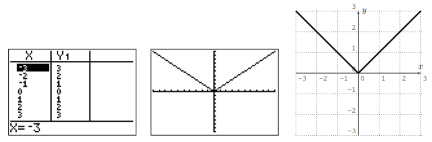
We have drawn the graph a second time in the $x$-$y$-plane on the right.
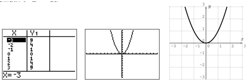
Similarly, we obtain the graph for $y=x^2$, which is a parabola. The domain is $D=\mathbb{R}$.
$clipboard_ebcaafa16e9bd9cc42254e4f6f8548480.png$
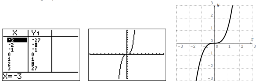
Here is the graph for $y=x^3$. The domain is $D=\mathbb{R}$.
$clipboard_e5ffcc4db19fb3579d76f969fe6484254.png$
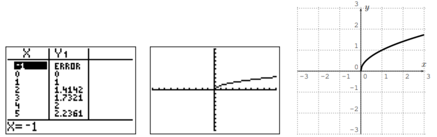
Next we graph $y=\sqrt{x}$. The domain is $D=[0,\infty)$.
$clipboard_e377eb0855dea55bb7701b94de2712656.png$
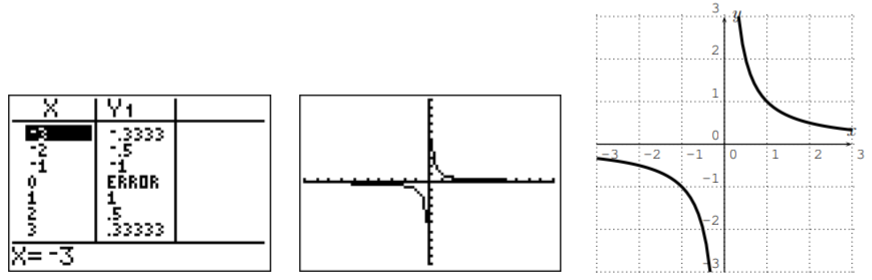
Finally, here is the graph for $y=\dfrac 1 x$. The domain is $D=\mathbb{R}-\{0\}$.
$clipboard_e8d0fd4adfd2afe42885f105f90739ec8.png$

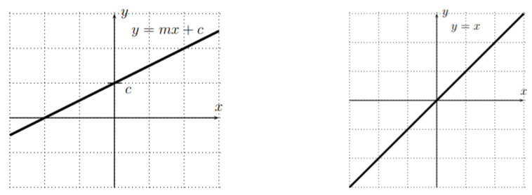
These graphs together with the line $y=mx+b$ studied in Section 2.1 are our basic building blocks for more complicated graphs in the next sections. Note in particular, that the graph of $y=x$ is the diagonal line.

$clipboard_e234f2ae225811f7972c52cd4ec1b4787.png$