11.2: Optional section- Rational functions by hand

Last updated
Save as PDF

Page ID: 49018

Thomas Tradler and Holly Carley
CUNY New York City College of Technology via New York City College of Technology at CUNY Academic Works

$ \newcommand{\vecs}[1]{\overset { \scriptstyle \rightharpoonup} {\mathbf{#1}} } $ $ \newcommand{\vecd}[1]{\overset{-\!-\!\rightharpoonup}{\vphantom{a}\smash {#1}}} $$\newcommand{\id}{\mathrm{id}}$ $ \newcommand{\Span}{\mathrm{span}}$ $ \newcommand{\kernel}{\mathrm{null}\,}$ $ \newcommand{\range}{\mathrm{range}\,}$ $ \newcommand{\RealPart}{\mathrm{Re}}$ $ \newcommand{\ImaginaryPart}{\mathrm{Im}}$ $ \newcommand{\Argument}{\mathrm{Arg}}$ $ \newcommand{\norm}[1]{\| #1 \|}$ $ \newcommand{\inner}[2]{\langle #1, #2 \rangle}$ $ \newcommand{\Span}{\mathrm{span}}$ $\newcommand{\id}{\mathrm{id}}$ $ \newcommand{\Span}{\mathrm{span}}$ $ \newcommand{\kernel}{\mathrm{null}\,}$ $ \newcommand{\range}{\mathrm{range}\,}$ $ \newcommand{\RealPart}{\mathrm{Re}}$ $ \newcommand{\ImaginaryPart}{\mathrm{Im}}$ $ \newcommand{\Argument}{\mathrm{Arg}}$ $ \newcommand{\norm}[1]{\| #1 \|}$ $ \newcommand{\inner}[2]{\langle #1, #2 \rangle}$ $ \newcommand{\Span}{\mathrm{span}}$$\newcommand{\AA}{\unicode[.8,0]{x212B}}$

In this section we will show how to sketch the graph of a factored rational function without the use of a calculator. It will be helpful to the reader to have read section 3 on graphing a polynomial by hand before continuing in this section. In addition to having the same difficulties as polynomials, calculators often have difficulty graphing rational functions near an asymptote.

Example $\PageIndex{1}$

Graph the function $p(x)=\dfrac{-3x^2(x-2)^3(x+2)}{(x-1)(x+1)^2(x-3)^3}$.

Solution

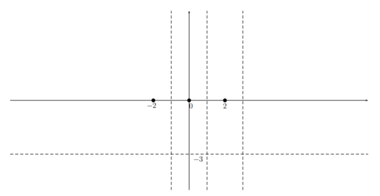
We can see that $p$ has zeros at $x=0,2,$ and $-2$ and vertical asymptotes $x=1$, $x=-1$ and $x=3$. Also note that for large $|x|$, $p(x)\approx -3$. So there is a horizontal asymptote $y=-3$. We indicate each of these facts on the graph:

$clipboard_e1ab5cc017086ae6ddfbc5b1e97a886ca.png$

We can in fact get a more precise statement by performing a long division and writing $p(x)=\dfrac{n(x)}{d(x)}= -3+\dfrac{r(x)}{d(x)}$. If you drop all but the leading order terms in the numerator and the denominator of the second term, we see that $p(x)\approx -3-\frac{12}{x}$ whose graph for large $|x|$ looks like

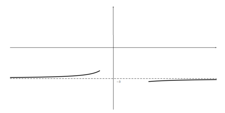
$clipboard_ec38d2a7bd99fe6baace384781d7e058b.png$

This sort of reasoning can make the graph a little more accurate but is not necessary for a sketch.

We also have the following table:

\[\begin{array}{r|l|l|l}
\text { for } a & \text { near } a, p(x) \approx & \text { type } & \text { sign change at } a \\
\hline-2 & C_{1}(x+2) & \text { linear } & \text { changes } \\
-1 & C_{2} /(x+1)^{2} & \text { asymptote } & \text { does not change } \\
0 & C_{3} x^{2} & \text { parabola } & \text { does not change } \\
1 & C_{4} /(x-1) & \text { asymptote } & \text { changes } \\
2 & C_{5}(x-2)^{3} & \text { cubic } & \text { changes } \\
3 & C_{6} /(x-3)^{3} & \text { asymptote } & \text { changes }
\end{array} \nonumber \]

Note that if the power appearing in the second column is even then the function does not change from one side of $a$ to the other. If the power is odd, the sign changes (either from positive to negative or from negative to positive).

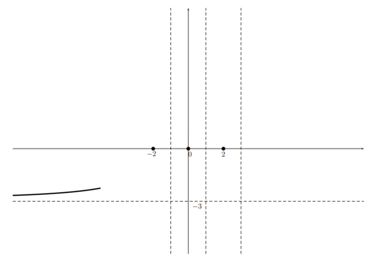
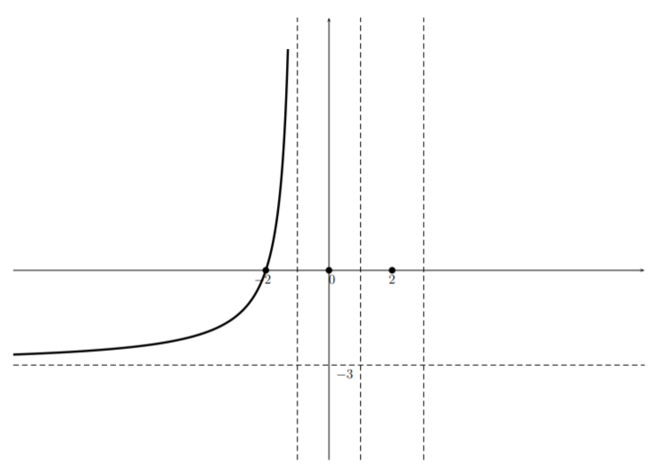
Now we move from large negative $x$ values toward the right, taking into account the above table. For large negative $x$, we start our sketch as follows:

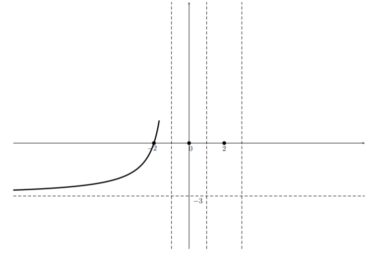
$clipboard_ec81bedade4b6eda8f6ade524b3e1e6af.png$

And noting that near $x=-2$ the function $p(x)$ is approximately linear, we have

$clipboard_e989926d8794a318a3cefea902bc0570c.png$

Then noting that we have an asymptote (noting that we can not cross the $x$-axis without creating an $x$-intercept) we have

$clipboard_e04a2ea647dacaef54850fb4154e2331c.png$

Now, from the table we see that there is no sign change at $-1$ so we have

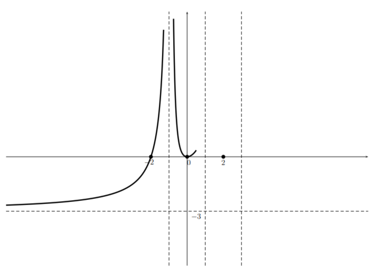
$clipboard_e9e714f40cc75354c84e362afd3b3a8dd.png$

and from the table we see that near $x=0$ the function $p(x)$ is approximately quadratic and therefore the graph looks like a parabola. This together with the fact that there is an asymptote at $x=1$ gives

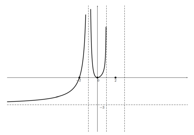
$clipboard_efc1a9a9350a0e803a3a050301a3b7811.png$

Now, from the table we see that the function changes sign at the asymptote, so while the graph “hugs” the top of the asymptote on the left hand side, it “hugs” the bottom on the right hand side giving

$clipboard_e0d63cea5abaf6524dc049fffda77d4b3.png$

Now, from the table we see that near $x=2$, $p(x)$ is approximately cubic. Also, there is an asymptote $x=3$ so we get

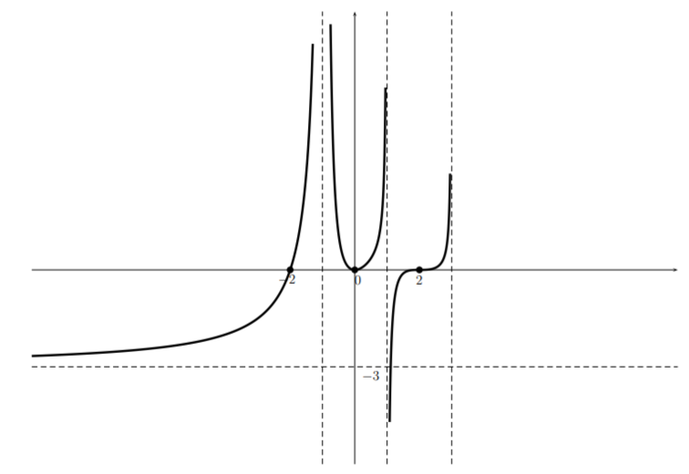
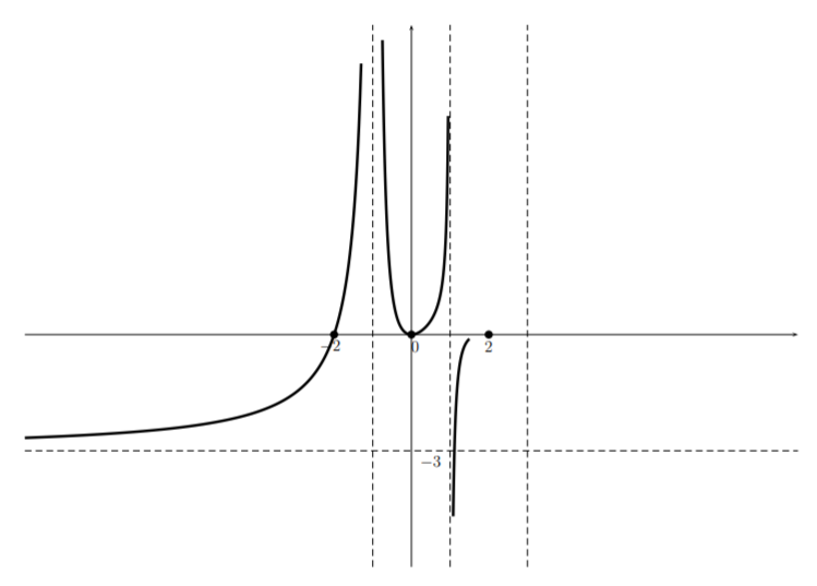
$clipboard_e49f2ce397ee19fd103adfd949b53cbc3.png$

Finally, we see from the table that $p(x)$ changes sign at the asymptote $x=3$ and has a horizontal asymptote $y=-3$, so we complete the sketch:

$clipboard_ed49fe558b902b221b968d4e526646c6b.png$

Note that if we had made a mistake somewhere there is a good chance that we would have not been able to get to the horizontal asymptote on the right side without creating an additional $x$-intercept.

What can we conclude from this sketch? This sketch exhibits only the general shape which can help decide on an appropriate window if we want to investigate details using technology. Furthermore, we can infer where $p(x)$ is positive and where $p(x)$ is negative. However, it is important to notice, that there may be wiggles in the graph that we have not included in our sketch.

We now give one more example of graphing a rational function where the horizontal asymptote is $y=0$.

Example $\PageIndex{2}$

Sketch the graph of \[r(x)=\dfrac{2x^2(x-1)^3(x+2)}{(x+1)^4(x-2)^3} \nonumber \]

Solution

Here we see that there are $x$-intercepts at $(0,0)$, $(0,1)$, and $(0,-2)$. There are two vertical asymptotes: $x=-1$ and $x=2$. In addition, there is a horizontal asymptote at $y=0$. (Why?) Putting this information on the graph gives

$clipboard_e4f859389afc0f55141632cd6fb48f000.png$

In this case, it is easy to get more information for large $|x|$ that will be helpful in sketching the function. Indeed, when $|x|$ is large, we can approximate $r(x)$ by dropping all but the highest order term in the numerator and denominator which gives $r(x)\approx\dfrac{2x^6}{x^7}=\frac{2}{x}$. So for large $|x|$, the graph of $r$ looks like

$clipboard_e6d8053242b9025eb3893ad0d3846e40f.png$

The function gives the following table:

\[\begin{array}{r|l|l|l}
\text { for } a & \text { near } a, p(x) \approx & \text { type } & \text { sign change at } a \\
\hline-2 & C_{1}(x+2) & \text { linear } & \text { changes } \\
-1 & C_{2} /(x+1)^{4} & \text { asymptote } & \text { does not change } \\
0 & C_{3} x^{2} & \text { parabola } & \text { does not change } \\
1 & C_{4}(x-1)^{3} & \text { cubic } & \text { changes } \\
2 & C_{5} /(x-2)^{3} & \text { asymptote } & \text { changes }
\end{array} \nonumber \]

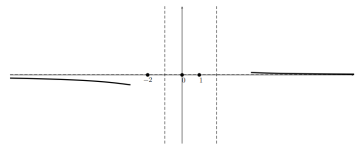
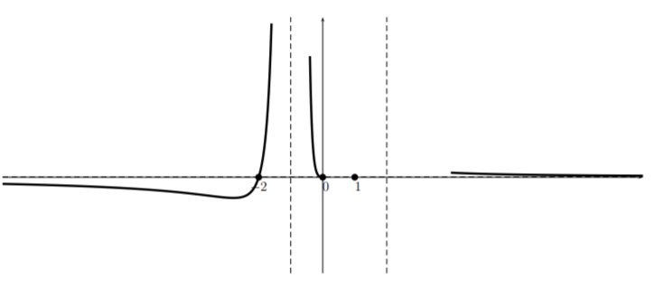
Looking at the table for this function, we see that the graph should look like a line near the zero $(0,-2)$ and since it has an asymptote $x=-1$, the graph looks something like:

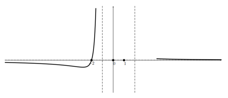
$clipboard_e3750fd92635a6d8bdc1c8744b304474c.png$

Then, looking at the table we see that $r(x)$ does not change its sign near $x=-1$, so that we obtain:

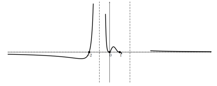
$clipboard_e02cc987f68f398981d1e61fea94e2212.png$

Now, the function is approximately quadratic near $x=0$ so the graph looks like:

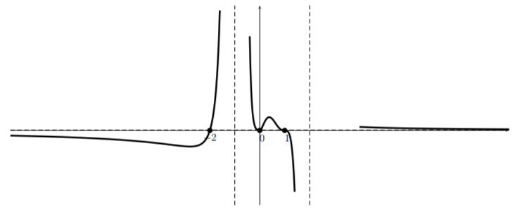
$clipboard_e1df40fffe76ea770a397737b676373c1.png$

Turning to head toward the root at $1$ and noting that the function is approximately cubic there, and that there is an asymptote $x=2$, we have:

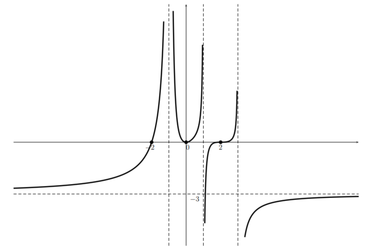
$clipboard_e5a4f325fb48371afe146bc8194317af8.png$

Finally, we see that the function changes sign at $x=2$ (see the table). So since the graph “hugs” the asymptote near the bottom of the graph on the left side of the asymptote, it will “hug” the asymptote near the top on the right side. So this together with the fact that $y=0$ is an asymptote gives the sketch (perhaps using an eraser to match the part of the graph on the right that uses the large $x$):

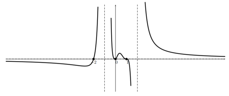
$clipboard_e93dd677eac58d09310564e3ba5b17f65.png$

Note that if the graph couldn’t be matched at the end without creating an extra $x$-intercept, then a mistake has been made.