11.1: Graphs of rational functions

Recall from the beginning of this chapter that a rational function is a fraction of polynomials:

\[f(x)=\dfrac{a_n x^n+a_{n-1}x^{n-1}+\dots+a_1 x+a_0}{b_m x^m+b_{m-1}x^{m-1}+\dots+b_1 x+b_0} \nonumber \]

In this section, we will study some characteristics of graphs of rational functions. Asymptotes are important features of graphs of rational functions. An asymptote is a line that is approached by the graph of a function: \(x=a\) is a vertical asymptote if \(f(x)\) approaches \(\pm \infty\) as \(x\) approaches \(a\) from either the left or from the right, and \(y=b\) is a horizontal asymptote if \(f(x)\) approaches \(b\) as \(x\) approaches \(\infty\) or \(-\infty\).

To obtain a better idea of some of these features including asymptotes, we start by graphing some rational functions. In particular it is useful to know the graphs of the basic functions \(y=\dfrac 1 {x^n}\).

Observation: Asymptotes

Graphing \(y=\dfrac 1 {x}\), \(y=\dfrac 1 {x^2}\), \(y=\dfrac 1 {x^3}\), \(y=\dfrac 1 {x^4}\), we obtain:

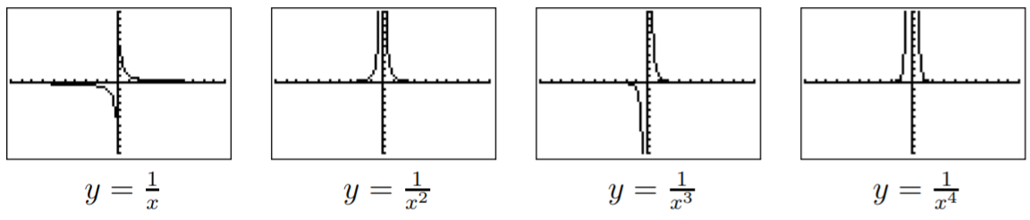
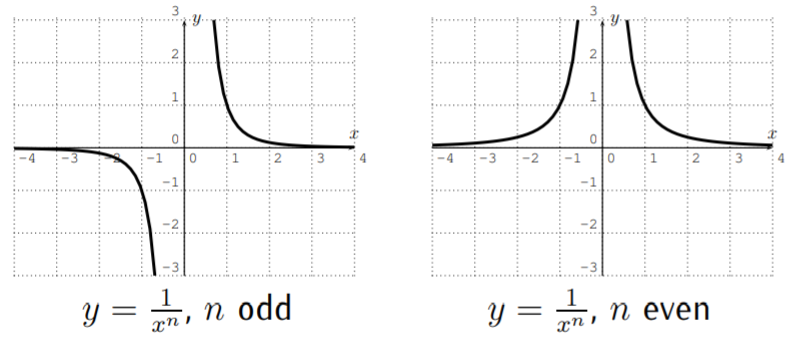
In general we see that \(x=0\) is a vertical asymptote and \(y=0\) is a horizontal asymptote. The shape of \(y=\dfrac 1 {x^n}\) depends on \(n\) being even or odd. We have:

We now study more general rational functions.

Example \(\PageIndex{1}\)

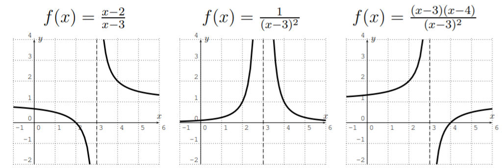
1. Our first graph is \(f(x)=\dfrac 1 {x-3}\).

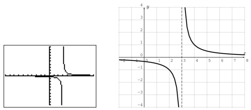
Here, the domain is all numbers where the denominator is not zero, that is \(D=\mathbb{R}-\{3\}\). There is a vertical asymptote, \(x=3\). Furthermore, the graph approaches \(0\) as \(x\) approaches \(\pm \infty\). Therefore, \(f\) has a horizontal asymptote, \(y=0\). Indeed, whenever the denominator has a higher degree than the numerator, the line \(y=0\) will be the horizontal asymptote.

2. Next, we graph \(f(x)=\dfrac{8x^2-8}{4x^2-16}\).

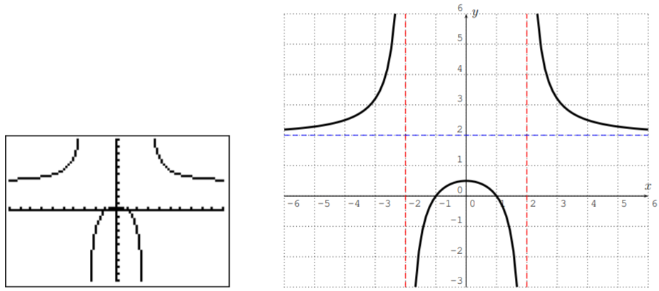
Here, the domain is all \(x\) for which \(4x^2-16\neq 0\). To see where this happens, calculate

\[4x^2-16=0 \implies \quad 4x^2=16 \implies\quad x^2=4 \implies\quad x=\pm 2 \nonumber \]

Therefore, the domain is \(D=\mathbb{R}-\{-2,2\}\). As before, we see from the graph, that the domain reveals the vertical asymptotes \(x=2\) and \(x=-2\) (the vertical dashed lines). To find the horizontal asymptote (the horizontal dashed line), we note that when \(x\) becomes very large, the highest terms of both numerator and denominator dominate the function value, so that

\[\text{for $|x|$ very large } \implies \quad f(x)=\dfrac{8x^2-8}{4x^2-16}\approx \dfrac{8x^2}{4x^2}=2 \nonumber \]

Therefore, when \(x\) approaches \(\pm\infty\), the function value \(f(x)\) approaches \(2\), and therefore the horizontal asymptote is at \(y=2\) (the horizontal dashed line).

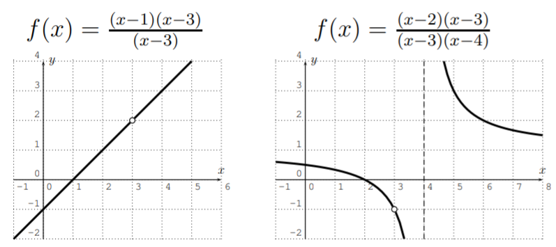
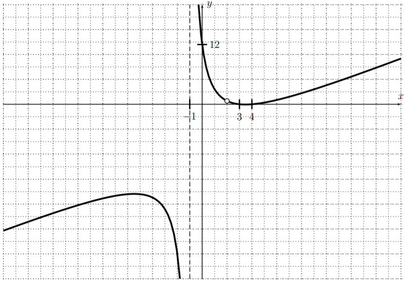
3. Our next graph is \(f(x)=\dfrac{x^2-8x+15}{x-3}\).

We see that there does not appear to be any vertical asymptote, despite the fact that \(3\) is not in the domain. The reason for this is that we can “remove the singularity” by cancelling the troubling term \(x-3\) as follows:

\[f(x)=\dfrac{x^2-8x+15}{x-3}=\dfrac{(x-3)(x-5)}{(x-3)}=\dfrac{x-5}{1}=x-5,\quad x\not=3 \nonumber \]

Therefore, the function \(f\) reduces to \(x-5\) for all values where it is defined. However, note that \(f(x)=\dfrac{x^2-8x+15}{x-3}\) is not defined at \(x=3\). We denote this in the graph by an open circle at \(x=3\), and call this a removable singularity (or a hole).

4. Our fourth and last graph before stating the rules in full generality is \(f(x)=\dfrac{2x^3-8}{3x^2-16}\).

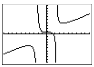
The graph indicates that there is no horizontal asymptote, as the graph appears to increase towards \(\infty\) and decrease towards \(-\infty\). To make this observation precise, we calculate the behavior when \(x\) approaches \(\pm \infty\) by ignoring the lower terms in the numerator and denominator

\[\text{for $|x|$ very large } \implies \quad f(x)=\dfrac{2x^3-8}{3x^2-16}\approx \dfrac{2x^3}{3x^2}=\dfrac{2x}{3} \nonumber \]

Therefore, when \(x\) becomes very large, \(f(x)\) behaves like \(\dfrac{2}{3}x\), which approaches \(\infty\) when \(x\) approaches \(\infty\), and approaches \(-\infty\) when \(x\) approaches \(-\infty\). (In fact, after performing a long division we obtain \(\dfrac{2x^3-8}{3x^2-16}=\dfrac{2}{3}\cdot x+\dfrac{r(x)}{3x^2-16}\), which would give rise to what is called a slant asymptote \(y=\dfrac{2}{3}\cdot x\); see also Note: Asymptotic Behaviour below.) Indeed, whenever the degree of the numerator is greater than the degree of the denominator, we find that there is no horizontal asymptote, but the graph blows up to \(\pm\infty\). (Compare this also with example (c) above).

Combining what we have learned from the above examples, we state our observations as follows.

Observation: Word

Let \(f(x)=\dfrac{p(x)}{q(x)}\) be a rational function with polynomials \(p(x)\) and \(q(x)\) in the numerator and denominator, respectively.

• The domain of \(f\) is all real numbers \(x\) for which the denominator is not zero, \[D=\{\quad x\in \mathbb{R} \quad|\quad q(x)\neq 0\quad \} \nonumber \]
• Assume that \(q(x_0)=0\), so that \(f\) is not defined at \(x_0\). If \(x_0\) is not a root of \(p(x)\), or if \(x_0\) is a root of \(p(x)\) but of a lesser multiplicity than the root in \(q(x)\), then \(f\) has a vertical asymptote \(x=x_0\).

• If \(p(x_0)=0\) and \(q(x_0)=0\), and the multiplicity of the root \(x_0\) in \(p(x)\) is at least the multiplicity of the root in \(q(x)\), then these roots can be canceled, and it is said that there is a removable discontinuity (or sometimes called a hole) at \(x=x_0\).

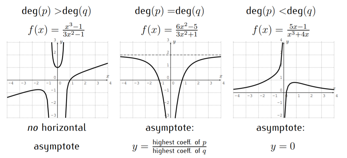
• To find the horizontal asymptotes, we need to distinguish the cases where the degree of \(p(x)\) is less than, equal to, or greater than \(q(x)\).

In addition, it is sometimes useful to determine the \(x\)- and \(y\)-intercepts.

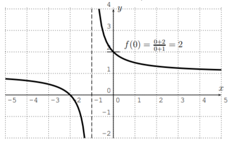
• If \(0\) is in the domain of \(f\), then the \(y\)-intercept is \((0,f(0))\). \[f(x)=\dfrac{x+2}{x+1} \nonumber \]

• If \(p(x_0)=0\) but \(q(x_0)\neq 0\), then \(f(x_0)=\dfrac{p(x_0)}{q(x_0)}=\dfrac{0}{q(x_0)}=0\), so that \((x_0,0)\) is an \(x\)-intercept, that is the graph intersects with the \(x\)-axis at \(x_0\). &&

\(f(x)=\dfrac{x-2}{x-3}\)

\(f(x)=\dfrac{(x-2)(x-4)(x-5)}{(x-3)^3}\)

Note: Asymptotic Behaviour

We can calculate the asymptotic behavior of a rational function \(f(x)=\dfrac{p(x)}{q(x)}\) in the case where the degree of \(p\) is greater than the degree of \(q\) by performing a long division. If the the quotient is \(m(x)\), and the remainder is \(r(x)\), then

\[f(x)=\dfrac{p(x)}{q(x)}=m(x)+\dfrac{r(x)}{q(x)} \nonumber \]

Now, since deg\((r)<\)deg\((q)\), the fraction \(\dfrac{r(x)}{q(x)}\) approaches zero as \(x\) approaches \(\pm\infty\), so that \(f(x)\approx m(x)\) for large \(x\).

Example \(\PageIndex{2}\)

Find the domain, all horizontal asymptotes, vertical asymptotes, removable singularities, and \(x\)- and \(y\)-intercepts. Use this information together with the graph of the calculator to sketch the graph of \(f\).

1. \(f(x)=\dfrac{-x^2}{x^2-3x-4}\)
2. \(f(x)=\dfrac{5x}{x^2-2x}\)
3. \(f(x)=\dfrac{x^3-9x^2+26x-24}{x^2-x-2}\)
4. \(f(x)=\dfrac{x-4}{(x-2)^2}\)
5. \(f(x)=\dfrac{3x^2-12}{2x^2+1}\)

Solution

1. We combine our knowledge of rational functions and its algebra with the particular graph of the function. The calculator gives the following graph.

To find the domain of \(f\) we only need to exclude from the real numbers those \(x\) that make the denominator zero. Since \(x^2-3x-4=0\) exactly when \((x+1)(x-4)=0\), which gives \(x=-1\) or \(x=4\), we have the domain:

\[\text{domain }D=\mathbb{R}-\{-1,4\} \nonumber \]

The numerator has a root exactly when \(-x^2=0\), that is \(x=0\). Therefore, \(x=-1\) and \(x=4\) are vertical asymptotes, and since we cannot cancel terms in the fraction, there is no removable singularity. Furthermore, since \(f(x)=0\) exactly when the numerator is zero, the only \(x\)-intercept is \((0,0)\).

To find the horizontal asymptote, we consider \(f(x)\) for large values of \(x\) by ignoring the lower order terms in numerator and denominator,

\[|x| \text{ large } \implies f(x)\approx \dfrac{-x^2}{x^2}=-1 \nonumber \]

We see that the horizontal asymptote is \(y=-1\). Finally, for the \(y\)-intercept, we calculate \(f(0)\):

\[f(0)=\dfrac{- 0^2}{0^2-3\cdot 0-4}=\dfrac{0}{-4}=0 \nonumber \]

Therefore, the \(y\)-intercept is \((0,0)\). The function is then graphed as follows.

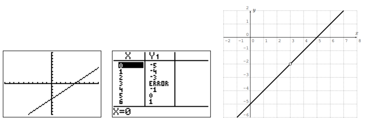
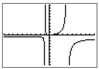
2. The graph of \(f(x)=\dfrac{5x}{x^2-2x}\) as drawn with the TI-84 is the following.

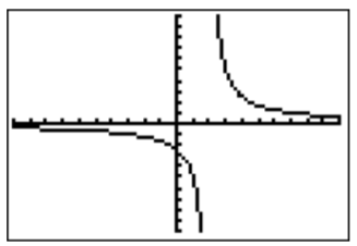
For the domain, we find the roots of the denominator,

\[x^2-2x=0 \implies \quad x (x-2)=0 \implies \quad x=0 \text{ or } x=2 \nonumber \]

The domain is \(D=\mathbb{R}-\{0,2\}\). For the vertical asymptotes and removable singularities, we calculate the roots of the numerator,

\[5x=0 \implies \quad x=0 \nonumber \]

Therefore, \(x=2\) is a vertical asymptote, and \(x=0\) is a removable singularity. Furthermore, the denominator has a higher degree than the numerator, so that \(y=0\) is the horizontal asymptote. For the \(y\)-intercept, we calculate \(f(0)\) by evaluating the fraction \(f(x)\) at \(0\)

\[\dfrac{5\cdot 0}{0^2-2\cdot 0}=\dfrac{0}{0} \nonumber \]

which is undefined. Therefore, there is no \(y\)-intercept (we, of course, already noted that there is a removable singularity when \(x=0\)). Finally for the \(x\)-intercept, we need to analyze where \(f(x)=0\), that is where \(5x=0\). The only candidate is \(x=0\) for which \(f\) is undefined. Again, we see that there is no \(x\)-intercept. The function is then graphed as follows. (Notice in particular the removable singularity at \(x=0\).)

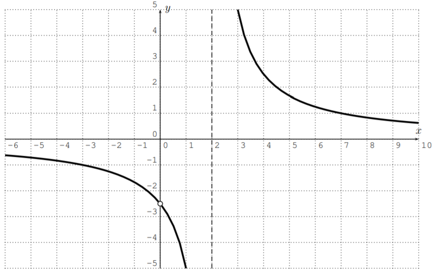
3. We start again by graphing the function \(f(x)=\dfrac{x^3-9x^2+26x-24}{x^2-x-2}\) with the calculator. After zooming to an appropriate window, we get:

To find the domain of \(f\), we find the zeros of the denominator

\[x^2-x-2=0 \implies\quad (x+1)(x-2)=0\implies \quad x=-1\text{ or }x=2 \nonumber \]

The domain is \(D=\mathbb{R}-\{-1,2\}\). The graph suggests that there is a vertical asymptote \(x=-1\). However the \(x=2\) appears not to be a vertical asymptote. This would happen when \(x=2\) is a removable singularity, that is, \(x=2\) is a root of both numerator and denominator of \(f(x)=\dfrac{p(x)}{q(x)}\). To confirm this, we calculate the numerator \(p(x)\) at \(x=2\):

\[p(2)=2^3-9\cdot 2^2+26 \cdot 2-24=8-36+52-24=0 \nonumber \]

Therefore, \(x=2\) is indeed a removable singularity. To analyze \(f\) further, we also factor the numerator. Using the factor theorem, we know that \(x-2\) is a factor of the numerator. Its quotient is calculated via long division.

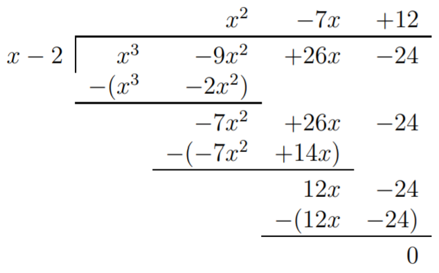
With this, we obtain

\[f(x)=\dfrac{(x-2)(x^2-7x+12)}{x^2-x-2}=\dfrac{(x-2)(x-3)(x-4)}{(x+1)(x-2)} \nonumber \]

Therefore, we conclude that \(x=-1\) is a vertical asymptote and \(x=2\) is a removable singularity. We also see that the \(x\)-intercepts are \((3,0)\) and \((4,0)\) (that is \(x-\) values where the numerator is zero).

Now, the long range behavior is determined by ignoring the lower terms in the fraction,

\[|x| \text{ large } \implies \quad f(x)\approx \dfrac{x^3}{x^2}=x \implies \quad \text{ no horizontal asymptote} \nonumber \]

Finally, the \(y\)-coordinate of the \(y\)-intercept is given by

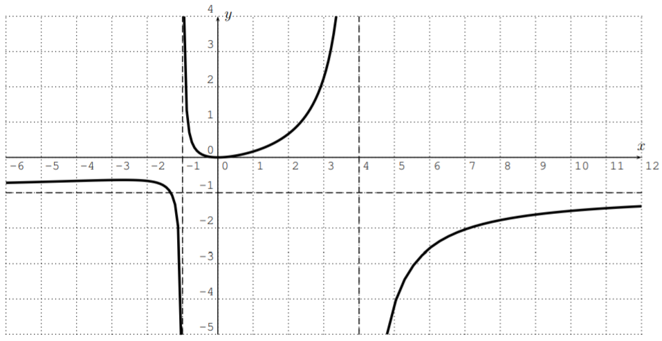
\[y=f(0)=\dfrac{0^3-9\cdot 0^2+26\cdot 0-24}{0^2-0-2}=\dfrac{-24}{-2}=12 \nonumber \]

We draw the graph as follows:

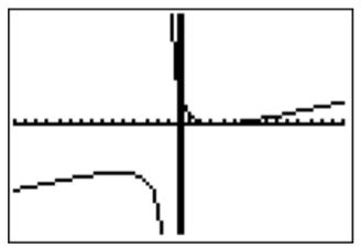
4. We first graph \(f(x)=\dfrac{x-4}{(x-2)^2}\). (Don’t forget to set the viewing window back to the standard settings!)

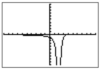
The domain is all real numbers except where the denominator becomes zero, that is, \(D=\mathbb{R}-\{2\}\). The graph has a vertical asymptote \(x=2\) and no hole. The horizontal asymptote is at \(y=0\), since the denominator has a higher degree than the numerator. The \(y\)-intercept is at \(y_0=f(0)=\dfrac{0-4}{(0-2)^2}=\dfrac{-4}{4}=-1\). The \(x\)-intercept is where the numerator is zero, \(x-4=0\), that is at \(x=4\). Since the above graph did not show the \(x\)-intercept, we can confirm this by changing the window size as follows:

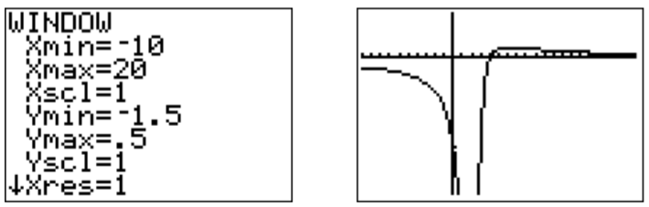
Note in particular that the graph intersects the \(x\)-axis at \(x=4\) and then changes its direction to approach the \(x\)-axis from above. A graph of the function \(f\) which includes all these features is displayed below.

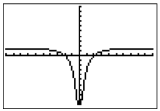
5. We graph \(f(x)=\dfrac{3x^2-12}{2x^2+1}\).

For the domain, we determine the zeros of the denominator.

\[2x^2+1=0\implies \quad 2x^2=-1\implies \quad x^2=-\dfrac{1}{2} \nonumber \]

The only solutions of this equation are given by complex numbers, but not by any real numbers. In particular, for any real number \(x\), the denominator of \(f(x)\) is not zero. The domain of \(f\) is all real numbers, \(D=\mathbb{R}\). This implies in turn that there are no vertical asymptotes, and no removable singularities.

The \(x\)-intercepts are determined by \(f(x)=0\), that is where the numerator is zero,

\[3x^2-12=0\implies \quad 3x^2=12\implies \quad x^2=4\implies \quad x=\pm 2 \nonumber \]

The horizontal asymptote is given by \(f(x)\approx\dfrac{3x^2}{2x^2}=\dfrac 3 2\), that is, it is at \(y=\dfrac 3 2=1.5\). The \(y\)-intercept is at

\[y=f(0)=\dfrac{3\cdot 0^2-12}{2\cdot 0^2+1}=\dfrac{-12}{1}=-12 \nonumber \]

We sketch the graph as follows:

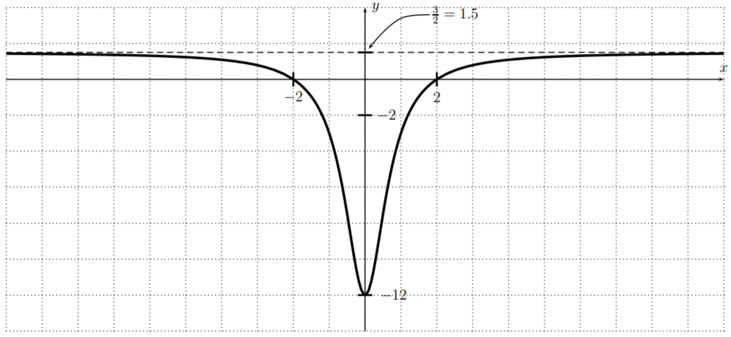
Since the graph is symmetric with respect to the \(y\)-axis, we can make one more observation, namely that the function \(f\) is even (see Observation: Even-Odd on page ):

\[f(-x)=\dfrac{3(-x)^2-12}{2(-x)^2+1}=\dfrac{3x^2-12}{2x^2+1}=f(x) \nonumber \]