13.1: Exponential functions and their graphs


- Last updated
- May 2, 2022
- Save as PDF

( \newcommand{\kernel}{\mathrm{null}\,}\)
We now consider functions that differ a great deal from polynomials and rational fractions in their complexity. More precisely, we will explore exponential and logarithmic functions from a function theoretic point of view. We start by recalling the definition of exponential functions and by studying their graphs.
A function f is called an exponential function if it is of the form f(x)=c⋅bx for some real number c and positive real number b. The constant b is called the base.
Graph the functions
f(x)=2x,g(x)=3x,h(x)=10x,k(x)=(12)x,l(x)=(110)x
Solution
First, we will graph the function f(x)=2x by calculating the function values in a table and then plotting the points in the x-y-plane. We can calculate the values by hand, or simply use the table function of the calculator to find the function values.
f(0)=20=1f(1)=21=2f(2)=22=4f(3)=23=8f(−1)=2−1=0.5f(−2)=2−2=0.25
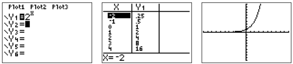
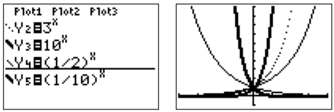
Similarly, we can calculate the table for the other functions g, h, k and l by entering the functions in the spots at Y2, Y3, Y4, and Y5. The values in the table for these functions can be seen by moving the cursor to the right with the ▹ key.

We can see the graphs by pressing the graph key.
In order to see these graphs more clearly, we adjust the graphing window to a more appropriate size.
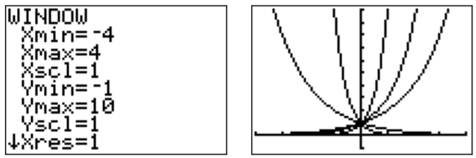
Since all these functions are graphed in the same window, it is difficult to associate the graphs with their corresponding functions. In order to distinguish between the graphs, we may use the TI-84 to draw the graphs in different line styles. In the function menu (y= ), move the cursor to the left with ◃, and press enter until the line becomes a thick line, or a dotted line, as desired. By moving the cursor down ▽, and pressing enter, we can adjust the line styles of the other graphs as well.
Note that the function k can also be written as k(x)=(12)x=(2−1)x=2−x and similarly, l(x)=(110)x=10−x.
This example shows that the exponential function has the following properties.
The graph of the exponential function f(x)=bx with b>0 and b≠1 has a horizontal asymptote at y=0.
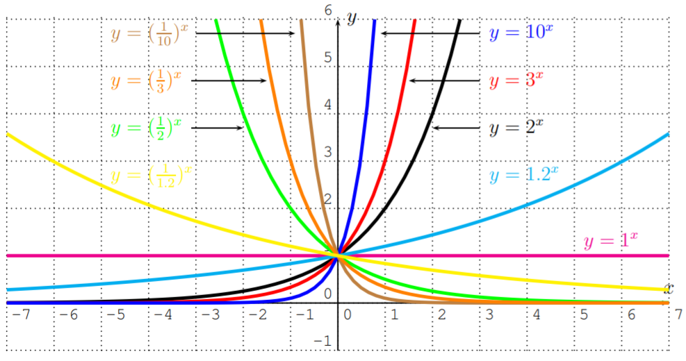
- If b>1, then f(x) approaches +∞ when x approaches +∞, and f(x) approaches 0 when x approaches −∞.
- If 0<b<1, then f(x) approaches 0 when x approaches +∞, and f(x) approaches +∞ when x approaches −∞.
An important base that we will frequently need to consider is the base of e, where e is the Euler number.
The Euler number e is an irrational number that is approximately
e=2.718281828459045235…
To be precise, we can define e as the number which is the horizontal asymptote of the function f(x)=(1+1x)x when x approaches +∞.
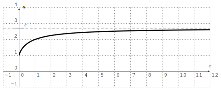
One can show that f has, indeed, a horizontal asymptote, and this limit is defined as e.
e:=limx→∞(1+1x)x
Furthermore, one can show that the exponential function with base e has a similar limit expression.
Alternatively, the Euler number and the exponential function with base e may also be defined using an infinite series, namely, er=1+r+r21⋅2+r31⋅2⋅3+r41⋅2⋅3⋅4+…. These ideas will be explored further in a course in calculus.
Graph the functions.
- y=ex
- y=e−x
- y=e−x2
- y=ex+e−x2
Solution
Using the calculator, we obtain the desired graphs. The exponential function y=ex may be entered via 2nd ln.
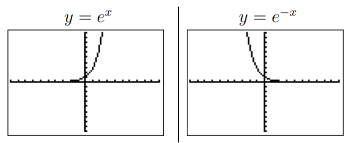
Note that the minus sign is entered in the last expression (and also in the following two functions) via the (−) key.

The last function y=ex+e−x2 is called the hyperbolic cosine, and is denoted by cosh(x)=ex+e−x2.
We now study how different multiplicative factors c affect the shape of an exponential function.
Graph the functions.
- y=2x
- y=3⋅2x
- y=(−3)⋅2x
- y=0.2⋅2x
- y=(−0.2)⋅2x
Solution
We graph the functions in one viewing window.
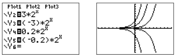
Here are the graphs of functions f(x)=c⋅2x for various choices of c.
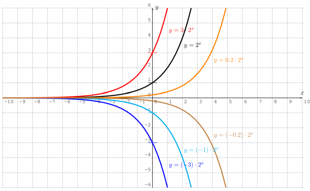
Note that for f(x)=c⋅2x, the y-intercept is given at f(0)=c.
Finally, we can combine our knowledge of graph transformations to study exponential functions that are shifted and stretched.
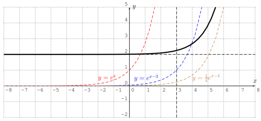
Graph the functions.
- y=3x−5
- y=ex+4
- y=14⋅ex−3+2
Solution
The graphs are displayed below.
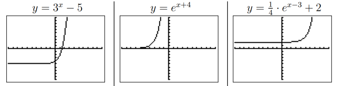
The first graph y=3x−5 is the graph of y=3x shifted down by 5.
The graph of y=ex+4 is the graph of y=ex shifted to the left by 4.
Finally, y=14ex−3+2 is the graph of y=ex shifted to the right by 3 (see the graph of y=ex−3), then compressed by a factor 4 towards the x-axis (see the graph of y=14ex−3), and then shifted up by 2.