7: Iterative Methods

Iterative methods are often used for solving a system of nonlinear equations. Even for linear systems, iterative methods have some advantages. They may require less memory and may be computationally faster. They are also easier to code. Here, without detailing the theoretical numerical analysis, we will simply explain the related iterative methods that go by the names of the Jacobi method, the Gauss-Seidel method, and the Successive Over Relaxation method (or SOR). We illustrate these three methods by showing how to solve the two-dimensional Poisson equation, an equation that we will later need to solve to determine the flow field past an obstacle

The Poisson equation is given by

$$-\nabla^{2} \Phi=f, \nonumber$$

where

$$\nabla^{2}=\frac{\partial^{2}}{\partial x^{2}}+\frac{\partial^{2}}{\partial y^{2}} \nonumber$$

is the usual two-dimensional Laplacian. This could be a linear equation with $f$ independent of $\Phi$, or a nonlinear equation where $f$ may be some nonlinear function of $\Phi$.

After discretizing the Poisson equation using the centered finite difference approximation for the second derivatives, we obtain on a grid with uniform grid spacing $h$,

$$4 \Phi_{i, j}-\Phi_{i+1, j}-\Phi_{i-1, j}-\Phi_{i, j+1}-\Phi_{i, j-1}=h^{2} f_{i, j} . \nonumber$$

The Jacobi method simply solves the discretized equation (7.1) for $\Phi_{i, j}$ iteratively. With superscripts indicating iteration steps, we have

$$\Phi_{i, j}^{(n+1)}=\frac{1}{4}\left(\Phi_{i+1, j}^{(n)}+\Phi_{i-1, j}^{(n)}+\Phi_{i, j+1}^{(n)}+\Phi_{i, j-1}^{(n)}+h^{2} f_{i, j}^{(n)}\right) . \nonumber$$

In the old FORTRAN-77 scientific programming language, implementing the Jacobi method required the saving of $\Phi$ in two different arrays, one corresponding to the $n$-th iteration, and one corresponding to the $(n+1)$-st iteration. When the iteration was done with a single array, the method was called Gauss-Seidel. In the standard Gauss-Seidel method, the array was updated row-by-row and had the form

$$\Phi_{i, j}^{(n+1)}=\frac{1}{4}\left(\Phi_{i+1, j}^{(n)}+\Phi_{i-1, j}^{(n+1)}+\Phi_{i, j+1}^{(n)}+\Phi_{i, j-1}^{(n+1)}+h^{2} f_{i, j}^{(n)}\right) . \nonumber$$

The Gauss-Seidel method had the double advantage of requiring less memory and converging more rapidly than the Jacobi method.

A variant of Gauss-Seidel that can also be found in textbooks is called red-black Gauss-Seidel. In this algorithm, the grid is viewed as a checkerboard with red and black squares. An updating of $\Phi_{i, j}$ is done in two passes: in the first pass, $\Phi_{i, j}$ is updated only on the red squares; in the second pass, only on the black squares. Because of the structure of the Laplacian finite difference operator, when solving $\nabla^{2} \Phi=0$ the updated values of $\Phi$ on the red squares depend only on the values of $\Phi$ on the black squares, and the updated values on the black squares depend only on the red squares.

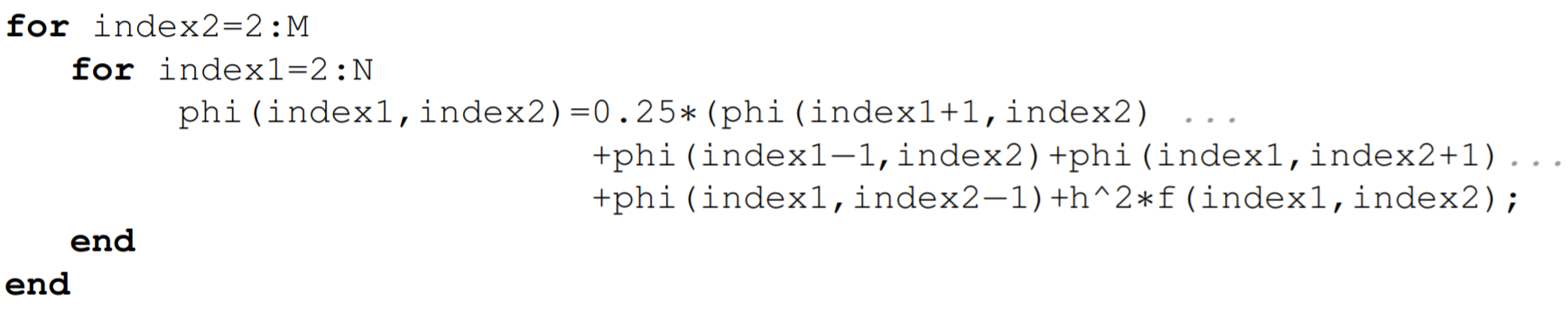
Translating FORTRAN-77 directly into MATLAB, the Gauss-Seidel method in the standard form could be implemented on a uniform grid with $N-1$ and $M-1$ internal grid points in the $x$-and $y$-directions, respectively, as

Nowadays, however, programming languages such as MATLAB operate on vectors, which are optimized for modern computers, and the explicit loops that used to be the workhorse of FORTRAN77 are now vectorized.

So to properly implement the Jacobi method, say, in MATLAB, one can predefine the vectors index 1 and index 2 that contain the index numbers of the first and second indices of the matrix variable phi. These definitions would be

where indexl and index 2 reference the internal grid points of the domain. The variable phi is assumed to be known on the boundaries of the domain corresponding to the indices $(1,1)$, $(N+1,1),(1, M+1)$, and $(N+1, M+1)$. The Jacobi method in MATLAB can then be coded in one line as

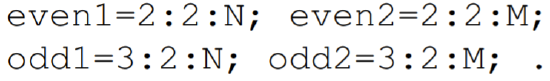
The red-black Gauss-Seidel method could be implemented in a somewhat similar fashion. One must now predefine the vectors even 1, odd1, even 2, and odd2, with definitions

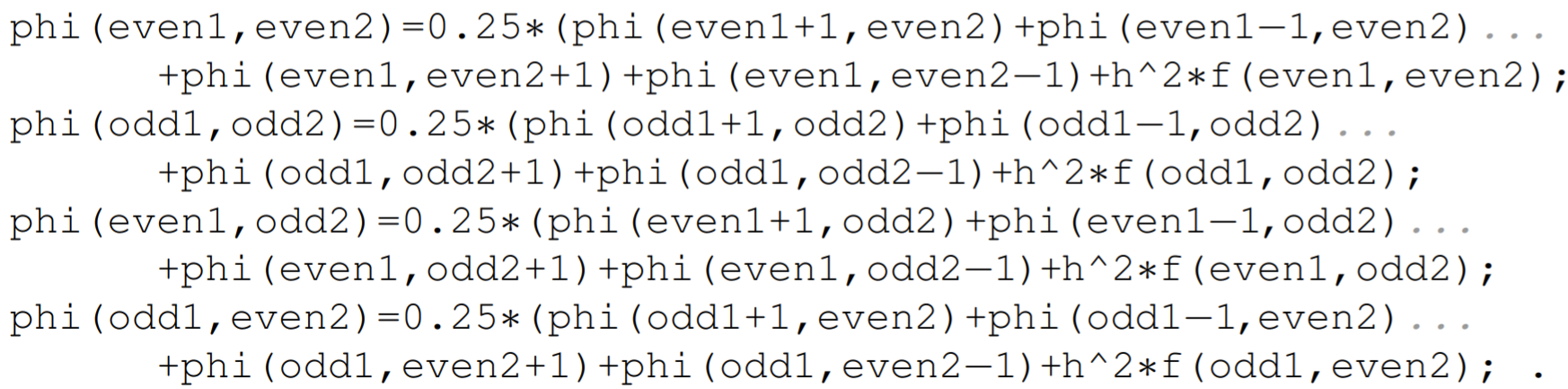
The red-black Gauss-Seidel method then requires the following four coding lines to implement:

Each iteration of the red-black Gauss-Seidel method will run slower than that of the Jacobi method, and the red-black Gauss-Seidel method will only be useful if the slower iterations are compensated by a faster convergence. In practice, however, the Jacobi method or the red-black Gauss Seidel method is replaced by the corresponding Successive Over Relaxation method (SOR method). We will illustrate this method using the Jacobi method, though the better approach is to use red-black Gauss-Seidel.

The Jacobi method is first rewritten by adding and subtracting the diagonal term $\Phi_{i, j}^{(n)}$ :

$$\Phi_{i, j}^{(n+1)}=\Phi_{i, j}^{(n)}+\frac{1}{4}\left(\Phi_{i+1, j}^{(n)}+\Phi_{i-1, j}^{(n)}+\Phi_{i, j+1}^{(n)}+\Phi_{i, j-1}^{(n)}-4 \Phi_{i, j}^{(n)}+h^{2} f_{i, j}^{(n)}\right) \nonumber$$

In this form, we see that the Jacobi method updates the value of $\Phi_{i, j}$ at each iteration. We can either magnify or diminish this update by introducing a relaxation parameter $\lambda$. We have

$$\Phi_{i, j}^{(n+1)}=\Phi_{i, j}^{(n)}+\frac{\lambda}{4}\left(\Phi_{i+1, j}^{(n)}+\Phi_{i-1, j}^{(n)}+\Phi_{i, j+1}^{(n)}+\Phi_{i, j-1}^{(n)}-4 \Phi_{i, j}^{(n)}+h^{2} f_{i, j}^{(n)}\right) \nonumber$$

which can be written more efficiently as

$$\Phi_{i, j}^{(n+1)}=(1-\lambda) \Phi_{i, j}^{(n)}+\frac{\lambda}{4}\left(\Phi_{i+1, j}^{(n)}+\Phi_{i-1, j}^{(n)}+\Phi_{i, j+1}^{(n)}+\Phi_{i, j-1}^{(n)}+h^{2} f_{i, j}^{(n)}\right) \nonumber$$

When used with Gauss-Seidel, a value of $\lambda$ in the range $1<\lambda<2$ can often be used to accelerate convergence of the iteration. When $\lambda>1$, the modifier over in Successive Over Relaxation is apt. When the right-hand-side of the Poisson equation is a nonlinear function of $\Phi$, however, the $\lambda=1$ Gauss-Seidel method may fail to converge. In this case, it may be reasonable to choose a value of $\lambda$ less than one, and perhaps a better name for the method would be Successive Under Relaxation. When under relaxing, the convergence of the iteration will of course be slowed. But this is the cost that must sometimes be paid for stability.

Newton’s method for a system of nonlinear equations

A system of nonlinear equations can be solved using a version of the iterative Newton’s Method for root finding. Although in practice, Newton’s method is often applied to a large nonlinear system, we will illustrate the method here for the simple system of two equations and two unknowns.

Suppose that we want to solve

$$f(x, y)=0, \quad g(x, y)=0, \nonumber$$

for the unknowns $x$ and $y$. We want to construct two simultaneous sequences $x_{0}, x_{1}, x_{2}, \ldots$ and $y_{0}, y_{1}, y_{2}, \ldots$ that converge to the roots. To construct these sequences, we Taylor series expand $f\left(x_{n+1}, y_{n+1}\right)$ and $g\left(x_{n+1}, y_{n+1}\right)$ about the point $\left(x_{n}, y_{n}\right) .$ Using the partial derivatives $f_{x}=$ $\partial f / \partial x, f_{y}=\partial f / \partial y$, etc., the two-dimensional Taylor series expansions, displaying only the linear terms, are given by

$$\begin{array}{ll} f\left(x_{n+1}, y_{n+1}\right)=f\left(x_{n}, y_{n}\right)+\left(x_{n+1}-x_{n}\right) f_{x}\left(x_{n}, y_{n}\right) & +\left(y_{n+1}-y_{n}\right) f_{y}\left(x_{n}, y_{n}\right)+\ldots \\ g\left(x_{n+1}, y_{n+1}\right)=g\left(x_{n}, y_{n}\right)+\left(x_{n+1}-x_{n}\right) g_{x}\left(x_{n}, y_{n}\right) & +\left(y_{n+1}-y_{n}\right) g_{y}\left(x_{n}, y_{n}\right)+\ldots . \end{array} \nonumber$$

To obtain Newton’s method, we take $f\left(x_{n+1}, y_{n+1}\right)=0, g\left(x_{n+1}, y_{n+1}\right)=0$, and drop higherorder terms above linear. Although one can then find a system of linear equations for $x_{n+1}$ and $y_{n+1}$, it is more convenient to define the variables

$$\Delta x_{n}=x_{n+1}-x_{n}, \quad \Delta y_{n}=y_{n+1}-y_{n} \nonumber$$

The iteration equations will then be given by

$$x_{n+1}=x_{n}+\Delta x_{n}, \quad y_{n+1}=y_{n}+\Delta y_{n} \nonumber$$

and the linear equations to be solved for $\Delta x_{n}$ and $\Delta y_{n}$ are given by

$$\left(\begin{array}{ll} f_{x} & f_{y} \\ g_{x} & g_{y} \end{array}\right)\left(\begin{array}{l} \Delta x_{n} \\ \Delta y_{n} \end{array}\right)=\left(\begin{array}{l} -f \\ -g \end{array}\right), \nonumber$$

where $f, g, f_{x}, f_{y}, g_{x}$, and $g_{y}$ are all evaluated at the point $\left(x_{n}, y_{n}\right) .$ The two-dimensional case is easily generalized to $n$ dimensions. The matrix of partial derivatives is called the Jacobian Matrix.

We illustrate Newton’s Method by finding numerically the steady state solution of the Lorenz equations, given by

$$\begin{aligned} \sigma(y-x) &=0, \\ r x-y-x z &=0, \\ x y-b z &=0, \end{aligned} \nonumber$$

where $x, y$, and $z$ are the unknown variables and $\sigma, r$, and $b$ are the known parameters. Here, we have a three-dimensional homogeneous system $f=0, g=0$, and $h=0$, with

$$\begin{aligned} &f(x, y, z)=\sigma(y-x), \\ &g(x, y, z)=r x-y-x z, \\ &h(x, y, z)=x y-b z . \end{aligned} \nonumber$$

The partial derivatives can be computed to be

$$\begin{array}{lll} f_{x}=-\sigma, & f_{y}=\sigma, & f_{z}=0, \\ g_{x}=r-z, & g_{y}=-1, & g_{z}=-x, \\ h_{x}=y, & h_{y}=x, & h_{z}=-b . \end{array} \nonumber$$

The iteration equation is therefore

$$\left(\begin{array}{ccc} -\sigma & \sigma & 0 \\ r-z_{n} & -1 & -x_{n} \\ y_{n} & x_{n} & -b \end{array}\right)\left(\begin{array}{c} \Delta x_{n} \\ \Delta y_{n} \\ \Delta z_{n} \end{array}\right)=-\left(\begin{array}{c} \sigma\left(y_{n}-x_{n}\right) \\ r x_{n}-y_{n}-x_{n} z_{n} \\ x_{n} y_{n}-b z_{n} \end{array}\right) \nonumber$$

with

$$\begin{aligned} &x_{n+1}=x_{n}+\Delta x_{n}, \\ &y_{n+1}=y_{n}+\Delta y_{n}, \\ &z_{n+1}=z_{n}+\Delta z_{n} . \end{aligned} \nonumber$$

The sample MATLAB program that solves this system is in the m-file newton_system.m.