10: The Simple Pendulum
- Page ID
- 93756

\( \newcommand{\vecs}[1]{\overset { \scriptstyle \rightharpoonup} {\mathbf{#1}} } \)
\( \newcommand{\vecd}[1]{\overset{-\!-\!\rightharpoonup}{\vphantom{a}\smash {#1}}} \)
\( \newcommand{\dsum}{\displaystyle\sum\limits} \)
\( \newcommand{\dint}{\displaystyle\int\limits} \)
\( \newcommand{\dlim}{\displaystyle\lim\limits} \)
\( \newcommand{\id}{\mathrm{id}}\) \( \newcommand{\Span}{\mathrm{span}}\)
( \newcommand{\kernel}{\mathrm{null}\,}\) \( \newcommand{\range}{\mathrm{range}\,}\)
\( \newcommand{\RealPart}{\mathrm{Re}}\) \( \newcommand{\ImaginaryPart}{\mathrm{Im}}\)
\( \newcommand{\Argument}{\mathrm{Arg}}\) \( \newcommand{\norm}[1]{\| #1 \|}\)
\( \newcommand{\inner}[2]{\langle #1, #2 \rangle}\)
\( \newcommand{\Span}{\mathrm{span}}\)
\( \newcommand{\id}{\mathrm{id}}\)
\( \newcommand{\Span}{\mathrm{span}}\)
\( \newcommand{\kernel}{\mathrm{null}\,}\)
\( \newcommand{\range}{\mathrm{range}\,}\)
\( \newcommand{\RealPart}{\mathrm{Re}}\)
\( \newcommand{\ImaginaryPart}{\mathrm{Im}}\)
\( \newcommand{\Argument}{\mathrm{Arg}}\)
\( \newcommand{\norm}[1]{\| #1 \|}\)
\( \newcommand{\inner}[2]{\langle #1, #2 \rangle}\)
\( \newcommand{\Span}{\mathrm{span}}\) \( \newcommand{\AA}{\unicode[.8,0]{x212B}}\)
\( \newcommand{\vectorA}[1]{\vec{#1}} % arrow\)
\( \newcommand{\vectorAt}[1]{\vec{\text{#1}}} % arrow\)
\( \newcommand{\vectorB}[1]{\overset { \scriptstyle \rightharpoonup} {\mathbf{#1}} } \)
\( \newcommand{\vectorC}[1]{\textbf{#1}} \)
\( \newcommand{\vectorD}[1]{\overrightarrow{#1}} \)
\( \newcommand{\vectorDt}[1]{\overrightarrow{\text{#1}}} \)
\( \newcommand{\vectE}[1]{\overset{-\!-\!\rightharpoonup}{\vphantom{a}\smash{\mathbf {#1}}}} \)
\( \newcommand{\vecs}[1]{\overset { \scriptstyle \rightharpoonup} {\mathbf{#1}} } \)
\(\newcommand{\longvect}{\overrightarrow}\)
\( \newcommand{\vecd}[1]{\overset{-\!-\!\rightharpoonup}{\vphantom{a}\smash {#1}}} \)
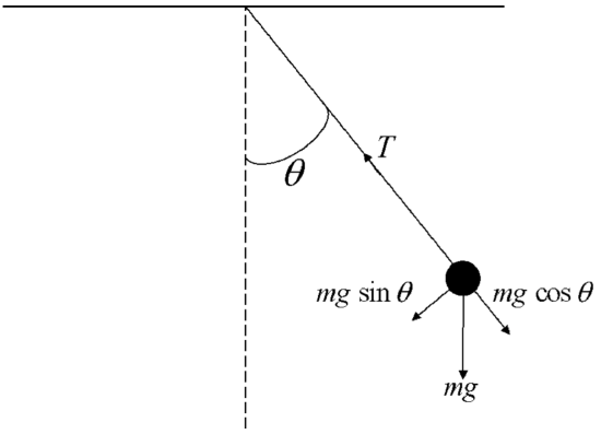
\(\newcommand{\avec}{\mathbf a}\) \(\newcommand{\bvec}{\mathbf b}\) \(\newcommand{\cvec}{\mathbf c}\) \(\newcommand{\dvec}{\mathbf d}\) \(\newcommand{\dtil}{\widetilde{\mathbf d}}\) \(\newcommand{\evec}{\mathbf e}\) \(\newcommand{\fvec}{\mathbf f}\) \(\newcommand{\nvec}{\mathbf n}\) \(\newcommand{\pvec}{\mathbf p}\) \(\newcommand{\qvec}{\mathbf q}\) \(\newcommand{\svec}{\mathbf s}\) \(\newcommand{\tvec}{\mathbf t}\) \(\newcommand{\uvec}{\mathbf u}\) \(\newcommand{\vvec}{\mathbf v}\) \(\newcommand{\wvec}{\mathbf w}\) \(\newcommand{\xvec}{\mathbf x}\) \(\newcommand{\yvec}{\mathbf y}\) \(\newcommand{\zvec}{\mathbf z}\) \(\newcommand{\rvec}{\mathbf r}\) \(\newcommand{\mvec}{\mathbf m}\) \(\newcommand{\zerovec}{\mathbf 0}\) \(\newcommand{\onevec}{\mathbf 1}\) \(\newcommand{\real}{\mathbb R}\) \(\newcommand{\twovec}[2]{\left[\begin{array}{r}#1 \\ #2 \end{array}\right]}\) \(\newcommand{\ctwovec}[2]{\left[\begin{array}{c}#1 \\ #2 \end{array}\right]}\) \(\newcommand{\threevec}[3]{\left[\begin{array}{r}#1 \\ #2 \\ #3 \end{array}\right]}\) \(\newcommand{\cthreevec}[3]{\left[\begin{array}{c}#1 \\ #2 \\ #3 \end{array}\right]}\) \(\newcommand{\fourvec}[4]{\left[\begin{array}{r}#1 \\ #2 \\ #3 \\ #4 \end{array}\right]}\) \(\newcommand{\cfourvec}[4]{\left[\begin{array}{c}#1 \\ #2 \\ #3 \\ #4 \end{array}\right]}\) \(\newcommand{\fivevec}[5]{\left[\begin{array}{r}#1 \\ #2 \\ #3 \\ #4 \\ #5 \\ \end{array}\right]}\) \(\newcommand{\cfivevec}[5]{\left[\begin{array}{c}#1 \\ #2 \\ #3 \\ #4 \\ #5 \\ \end{array}\right]}\) \(\newcommand{\mattwo}[4]{\left[\begin{array}{rr}#1 \amp #2 \\ #3 \amp #4 \\ \end{array}\right]}\) \(\newcommand{\laspan}[1]{\text{Span}\{#1\}}\) \(\newcommand{\bcal}{\cal B}\) \(\newcommand{\ccal}{\cal C}\) \(\newcommand{\scal}{\cal S}\) \(\newcommand{\wcal}{\cal W}\) \(\newcommand{\ecal}{\cal E}\) \(\newcommand{\coords}[2]{\left\{#1\right\}_{#2}}\) \(\newcommand{\gray}[1]{\color{gray}{#1}}\) \(\newcommand{\lgray}[1]{\color{lightgray}{#1}}\) \(\newcommand{\rank}{\operatorname{rank}}\) \(\newcommand{\row}{\text{Row}}\) \(\newcommand{\col}{\text{Col}}\) \(\renewcommand{\row}{\text{Row}}\) \(\newcommand{\nul}{\text{Nul}}\) \(\newcommand{\var}{\text{Var}}\) \(\newcommand{\corr}{\text{corr}}\) \(\newcommand{\len}[1]{\left|#1\right|}\) \(\newcommand{\bbar}{\overline{\bvec}}\) \(\newcommand{\bhat}{\widehat{\bvec}}\) \(\newcommand{\bperp}{\bvec^\perp}\) \(\newcommand{\xhat}{\widehat{\xvec}}\) \(\newcommand{\vhat}{\widehat{\vvec}}\) \(\newcommand{\uhat}{\widehat{\uvec}}\) \(\newcommand{\what}{\widehat{\wvec}}\) \(\newcommand{\Sighat}{\widehat{\Sigma}}\) \(\newcommand{\lt}{<}\) \(\newcommand{\gt}{>}\) \(\newcommand{\amp}{&}\) \(\definecolor{fillinmathshade}{gray}{0.9}\)We first consider the simple pendulum shown in Fig. 10.1. A mass is attached to a massless rigid rod, and is constrained to move along an arc of a circle centered at the pivot point. Suppose \(l\) is the fixed length of the connecting rod, and \(\theta\) is the angle it makes with the vertical axis. We will derive the governing equations for the motion of the mass, and an equation which can be solved to determine the period of oscillation.
Governing equations
The governing equations for the pendulum are derived from Newton’s equation, \(F=m a .\) Because the pendulum is constained to move along an arc, we can write Newton’s equation directly for the displacement \(s\) of the pendulum along the arc with origin at the bottom and positive direction to the right.
The relevant force on the pendulum is the component of the gravitational force along the arc, and from Fig. \(10.1\) is seen to be
\[F_{g}=-m g \sin \theta, \nonumber \]
where the negative sign signifies a force acting along the negative \(s\) direction when \(0<\theta<\pi\), and the positive \(s\) direction when \(-\pi<\theta<0\).
Newton’s equation for the simple pendulum moving along the arc is therefore
\[m \ddot{s}=-m g \sin \theta . \nonumber \]
Now, the relationship between the arc length \(s\) and the angle \(\theta\) is given by \(s=l \theta\), and therefore \(\ddot{s}=l \ddot{\theta} .\) The simple pendulum equation can then be written in terms of the angle \(\theta\) as
\[\ddot{\theta}+\omega^{2} \sin \theta=0, \nonumber \]
with
\[\omega=\sqrt{g / l} \nonumber \]
The standard small angle approximation \(\sin \theta \approx \theta\) results in the well-known equation for the simple harmonic oscillator,
\[\ddot{\theta}+\omega^{2} \theta=0 . \nonumber \]
We have derived the equations of motion by supposing that the pendulum is constrained to move along the arc of a circle. Such a constraint is valid provided the pendulum mass is connected to a massless rigid rod. If the rod is replaced by a massless spring, say, then oscillations in the length of the spring can occur. Deriving the equations for this more general physical situation requires considering the vector form of Newton’s equation.
It is informative to construct the equivalent governing equations in polar coordinates. To do so, we form the complex coordinate \(z=x+i y\), and make use of the polar form for \(z\), given by
\[z=r e^{i \theta} . \nonumber \]
The governing equations then become
\[\frac{d^{2}}{d t^{2}}\left(r e^{i \theta}\right)=g-\frac{T}{m} e^{i \theta} \nonumber \]
The second derivative can be computed using the product and chain rules, and one finds
\[\frac{d^{2}}{d t^{2}}\left(r e^{i \theta}\right)=\left(\left(\ddot{r}-r \dot{\theta}^{2}\right)+i(r \ddot{\theta}+2 \dot{r} \dot{\theta})\right) e^{i \theta} . \nonumber \]
Dividing both sides of \((10.7)\) by \(e^{i \theta}\), we obtain
\[\left(\ddot{r}-r \dot{\theta}^{2}\right)+i(r \ddot{\theta}+2 \dot{r} \dot{\theta})=g e^{-i \theta}-\frac{T}{m} . \nonumber \]
The two governing equations in polar coordinates, then, are determined by equating the real parts and the imaginary parts of \((10.9)\), and we find
\[\begin{align} &\ddot{r}-r \dot{\theta}^{2}=g \cos \theta-\frac{T}{m} \\ &r \ddot{\theta}+2 \dot{r} \dot{\theta}=-g \sin \theta \end{align} \nonumber \]
If the connector is a rigid rod, as we initially assumed, then \(r=l, \dot{r}=0\), and \(\ddot{r}=0 .\) The first equation \((10.10)\) is then an equation for the tension \(T\) in the rod, and the second equation (10.11) reduces to our previously derived (10.3). If the connector is a spring, then Hooke’s law may be applied. Suppose the spring constant is \(k\) and the unstretched spring has length \(l\). Then
\[T=k(r-l) \nonumber \]
in \((10.10)\), and a pair of simultaneous second-order equations govern the motion. The stable equilibrium with the mass at rest at the bottom satisfies \(\theta=0\) and \(r=l+m g / k ;\) i.e., the spring is stretched to counterbalance the hanging mass.
Period of motion
In general, the period of the simple pendulum depends on the amplitude of its motion. For small amplitude oscillations, the simple pendulum equation \((10.3)\) reduces to the simple harmonic oscillator equation (10.5), and the period becomes independent of amplitude. The general solution of the simple harmonic oscillator equation can be written as
\[\theta(t)=A \cos (\omega t+\varphi) \nonumber \]
Initial conditions on \(\theta\) and \(\dot{\theta}\) determine \(A\) and \(\varphi\), and by redefining the origin of time, one can always choose \(\varphi=0\) and \(A>0\). With this choice, \(A=\theta_{m}\), the maximum amplitude of the pendulum, and the analytical solution of \((10.5)\) is
\[\theta(t)=\theta_{m} \cos \omega t \nonumber \]
where \(\omega\) is called the angular frequency of oscillation. The period of motion is related to the angular frequency by
\[T=2 \pi / \omega, \nonumber \]
and is independent of the amplitude \(\theta_{m}\).
If \(\sin \theta \approx \theta\) is no longer a valid approximation, then we need to solve the simple pendulum equation (10.3). We first derive a closed form analytical expression, and then explain how to compute a numerical solution.
Analytical solution
A standard procedure for solving unfamiliar differential equations is to try and determine some combination of variables that is independent of time. Here, we can multiply \((10.3)\) by \(\dot{\theta}\) to obtain
\[\dot{\theta} \ddot{\theta}+\omega^{2} \dot{\theta} \sin \theta=0 . \nonumber \]
Now,
\[\dot{\theta} \ddot{\theta}=\frac{d}{d t}\left(\frac{1}{2} \dot{\theta}^{2}\right), \quad \dot{\theta} \sin \theta=\frac{d}{d t}(-\cos \theta), \nonumber \]
so that \((10.16)\) can be written as
\[\frac{d}{d t}\left(\frac{1}{2} \dot{\theta}^{2}-\omega^{2} \cos \theta\right)=0 \nonumber \]
The combination of variables in the parenthesis is therefore independent of time and is called an integral of motion. It is also said to be conserved, and \((10.18)\) is called a conservation law. In physics, this integral of motion (multiplied by \(m l^{2}\) ) is identified with the energy of the oscillator.
The value of this integral of motion at \(t=0\) is given by \(-\omega^{2} \cos \theta_{m}\), so the derived conservation law takes the form
\[\frac{1}{2} \dot{\theta}^{2}-\omega^{2} \cos \theta=-\omega^{2} \cos \theta_{m}, \nonumber \]
which is a separable first-order differential equation.
We can compute the period of oscillation \(T\) as four times the time it takes for the pendulum to go from its initial height to the bottom. During this quarter cycle of oscillation, \(d \theta / d t<0\) so that from (10.19),
\[\frac{d \theta}{d t}=-\sqrt{2} \omega \sqrt{\cos \theta-\cos \theta_{m}} . \nonumber \]
After separating and integrating over a quarter period, we have
\[\int_{0}^{T / 4} d t=-\frac{\sqrt{2}}{2 \omega} \int_{\theta_{m}}^{0} \frac{d \theta}{\sqrt{\cos \theta-\cos \theta_{m}}} \nonumber \]
or
\[T=\frac{2 \sqrt{2}}{\omega} \int_{0}^{\theta_{m}} \frac{d \theta}{\sqrt{\cos \theta-\cos \theta_{m}}} \nonumber \]
We can transform this equation for the period into a more standard form using a trigonometric identity and a substitution. The trig-identity is the well-known half-angle formula for sin, given by
\[\sin ^{2}(\theta / 2)=\frac{1}{2}(1-\cos \theta) \nonumber \]
Using this identity, we write
\[\cos \theta=1-2 \sin ^{2}(\theta / 2), \quad \cos \theta_{m}=1-2 \sin ^{2}\left(\theta_{m} / 2\right) \nonumber \]
and substituting (10.24) into (10.19) results in
\[T=\frac{2}{\omega} \int_{0}^{\theta_{m}} \frac{d \theta}{\sqrt{\sin ^{2}\left(\theta_{m} / 2\right)-\sin ^{2}(\theta / 2)}} . \nonumber \]
We now define the constant
\[a=\sin \left(\theta_{m} / 2\right) \nonumber \]
and perform the substitution
\[\sin \phi=\frac{1}{a} \sin (\theta / 2) \nonumber \]
Developing this substitution, we have
\[\cos \phi d \phi=\frac{1}{2 a} \cos (\theta / 2) d \theta . \nonumber \]
Now,
\[\begin{aligned} \cos (\theta / 2) &=\sqrt{1-\sin ^{2}(\theta / 2)} \\ &=\sqrt{1-a^{2} \sin ^{2} \phi} \end{aligned} \nonumber \]
so that \((10.28)\) can be solved for \(d \theta\) :
\[d \theta=\frac{2 a \cos \phi}{\sqrt{1-a^{2} \sin ^{2} \phi}} d \phi . \nonumber \]
Using \((10.27)\), the domain of integration \(\theta \in\left[0, \theta_{m}\right]\) transforms into \(\phi \in[0, \pi / 2] .\) Therefore, substituting (10.27) and (10.29) into (10.25) results in the standard equation for the period given by
\[T=\frac{4}{\omega} \int_{0}^{\pi / 2} \frac{d \phi}{\sqrt{1-a^{2} \sin ^{2} \phi}} \nonumber \]
with \(a\) given by (10.26). The integral \(T=T(a)\) is called the complete elliptic integral of the first kind.
For small amplitudes of oscillation, it is possible to determine the leading-order dependence of the period on \(\theta_{m}\). Now \(a\) is given by \((10.26)\), so that a Taylor series to leading order yields
\[a^{2}=\frac{1}{4} \theta_{m}^{2}+\mathrm{O}\left(\theta_{m}^{4}\right) \nonumber \]
Similarly, the Taylor series expansion of the integrand of \((10.30)\) is given by
\[\begin{aligned} \frac{1}{\sqrt{1-a^{2} \sin ^{2} \phi}} &=1+\frac{1}{2} a^{2} \sin ^{2} \phi+\mathrm{O}\left(a^{4}\right) \\ &=1+\frac{1}{8} \theta_{m}^{2} \sin ^{2} \phi+\mathrm{O}\left(\theta_{m}^{4}\right) \end{aligned} \nonumber \]
Therefore, from (10.30),
\[T=\frac{4}{\omega} \int_{0}^{\pi / 2} d \phi\left(1+\frac{1}{8} \theta_{m}^{2} \sin ^{2} \phi\right)+\mathrm{O}\left(\theta_{m}^{4}\right) \nonumber \]
Using
\[\int_{0}^{\pi / 2} d \phi \sin ^{2} \phi=\frac{\pi}{4} \nonumber \]
we have
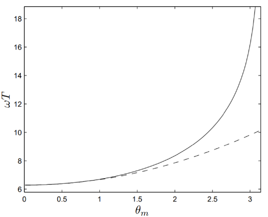
\[T=\frac{2 \pi}{\omega}\left(1+\frac{\theta_{m}^{2}}{16}\right)+\mathrm{O}\left(\theta_{m}^{4}\right) \nonumber \]
Numerical solution
We discuss here two methods for computing the period of the pendulum \(T=T\left(\theta_{m}\right)\) as a function of the maximum amplitude. The period can be found in units of \(\omega^{-1}\); that is, we compute \(\omega T\).
The first method makes use of our analytical work and performs a numerical integration of (10.30). Algorithms for numerical integration are discussed in Chapter 3 . In particular, use can be made of adaptive Simpson’s quadrature, implemented in the MATLAB function quad. \(\mathrm{m}\).
The second method, which is just as reasonable, solves the differential equation (10.3) directly. Nondimensionalizing using \(\tau=\omega t\), equation \((10.3)\) becomes
\[\frac{d^{2} \theta}{d \tau^{2}}+\sin \theta=0 \nonumber \]
To solve \((10.35)\), we write this second-order equation as the system of two first-order equations
\[\begin{aligned} &\frac{d \theta}{d \tau}=u, \\ &\frac{d u}{d \tau}=-\sin \theta, \end{aligned} \nonumber \]
with initial conditions \(\theta(0)=\theta_{m}\) and \(u(0)=0\). We then determine the (dimensionless) time required for the pendulum to move to the position \(\theta=0\) : this time will be equal to one-fourth of the period of motion
Algorithms for integration of ordinary differential equations are discussed in Chapter \(4 .\) In particular, use can be made of a Runge-Kutta \((4,5)\) formula, the Dormand-Prince pair, that is implemented in the MATLAB function ode \(45 . \mathrm{m}\).
Perhaps the simplest way to compute the period is to make use of the Event Location Property of the MATLAB ode solver. Through the odeset option, it is possible to instruct ode \(45 . \mathrm{m}\) to end the time integration when the event \(\theta=0\) occurs, and to return the time at which this event takes place.
A graph of the dimensionless period \(\omega T\) versus the amplitude \(\theta_{m}\) is shown in Fig. 10.2. For comparison, the low-order analytical result of \((10.34)\) is shown as the dashed line.