
12: Concepts and Tools
- Page ID
- 93758

\( \newcommand{\vecs}[1]{\overset { \scriptstyle \rightharpoonup} {\mathbf{#1}} } \)
\( \newcommand{\vecd}[1]{\overset{-\!-\!\rightharpoonup}{\vphantom{a}\smash {#1}}} \)
\( \newcommand{\dsum}{\displaystyle\sum\limits} \)
\( \newcommand{\dint}{\displaystyle\int\limits} \)
\( \newcommand{\dlim}{\displaystyle\lim\limits} \)
\( \newcommand{\id}{\mathrm{id}}\) \( \newcommand{\Span}{\mathrm{span}}\)
( \newcommand{\kernel}{\mathrm{null}\,}\) \( \newcommand{\range}{\mathrm{range}\,}\)
\( \newcommand{\RealPart}{\mathrm{Re}}\) \( \newcommand{\ImaginaryPart}{\mathrm{Im}}\)
\( \newcommand{\Argument}{\mathrm{Arg}}\) \( \newcommand{\norm}[1]{\| #1 \|}\)
\( \newcommand{\inner}[2]{\langle #1, #2 \rangle}\)
\( \newcommand{\Span}{\mathrm{span}}\)
\( \newcommand{\id}{\mathrm{id}}\)
\( \newcommand{\Span}{\mathrm{span}}\)
\( \newcommand{\kernel}{\mathrm{null}\,}\)
\( \newcommand{\range}{\mathrm{range}\,}\)
\( \newcommand{\RealPart}{\mathrm{Re}}\)
\( \newcommand{\ImaginaryPart}{\mathrm{Im}}\)
\( \newcommand{\Argument}{\mathrm{Arg}}\)
\( \newcommand{\norm}[1]{\| #1 \|}\)
\( \newcommand{\inner}[2]{\langle #1, #2 \rangle}\)
\( \newcommand{\Span}{\mathrm{span}}\) \( \newcommand{\AA}{\unicode[.8,0]{x212B}}\)
\( \newcommand{\vectorA}[1]{\vec{#1}} % arrow\)
\( \newcommand{\vectorAt}[1]{\vec{\text{#1}}} % arrow\)
\( \newcommand{\vectorB}[1]{\overset { \scriptstyle \rightharpoonup} {\mathbf{#1}} } \)
\( \newcommand{\vectorC}[1]{\textbf{#1}} \)
\( \newcommand{\vectorD}[1]{\overrightarrow{#1}} \)
\( \newcommand{\vectorDt}[1]{\overrightarrow{\text{#1}}} \)
\( \newcommand{\vectE}[1]{\overset{-\!-\!\rightharpoonup}{\vphantom{a}\smash{\mathbf {#1}}}} \)
\( \newcommand{\vecs}[1]{\overset { \scriptstyle \rightharpoonup} {\mathbf{#1}} } \)
\(\newcommand{\longvect}{\overrightarrow}\)
\( \newcommand{\vecd}[1]{\overset{-\!-\!\rightharpoonup}{\vphantom{a}\smash {#1}}} \)
\(\newcommand{\avec}{\mathbf a}\) \(\newcommand{\bvec}{\mathbf b}\) \(\newcommand{\cvec}{\mathbf c}\) \(\newcommand{\dvec}{\mathbf d}\) \(\newcommand{\dtil}{\widetilde{\mathbf d}}\) \(\newcommand{\evec}{\mathbf e}\) \(\newcommand{\fvec}{\mathbf f}\) \(\newcommand{\nvec}{\mathbf n}\) \(\newcommand{\pvec}{\mathbf p}\) \(\newcommand{\qvec}{\mathbf q}\) \(\newcommand{\svec}{\mathbf s}\) \(\newcommand{\tvec}{\mathbf t}\) \(\newcommand{\uvec}{\mathbf u}\) \(\newcommand{\vvec}{\mathbf v}\) \(\newcommand{\wvec}{\mathbf w}\) \(\newcommand{\xvec}{\mathbf x}\) \(\newcommand{\yvec}{\mathbf y}\) \(\newcommand{\zvec}{\mathbf z}\) \(\newcommand{\rvec}{\mathbf r}\) \(\newcommand{\mvec}{\mathbf m}\) \(\newcommand{\zerovec}{\mathbf 0}\) \(\newcommand{\onevec}{\mathbf 1}\) \(\newcommand{\real}{\mathbb R}\) \(\newcommand{\twovec}[2]{\left[\begin{array}{r}#1 \\ #2 \end{array}\right]}\) \(\newcommand{\ctwovec}[2]{\left[\begin{array}{c}#1 \\ #2 \end{array}\right]}\) \(\newcommand{\threevec}[3]{\left[\begin{array}{r}#1 \\ #2 \\ #3 \end{array}\right]}\) \(\newcommand{\cthreevec}[3]{\left[\begin{array}{c}#1 \\ #2 \\ #3 \end{array}\right]}\) \(\newcommand{\fourvec}[4]{\left[\begin{array}{r}#1 \\ #2 \\ #3 \\ #4 \end{array}\right]}\) \(\newcommand{\cfourvec}[4]{\left[\begin{array}{c}#1 \\ #2 \\ #3 \\ #4 \end{array}\right]}\) \(\newcommand{\fivevec}[5]{\left[\begin{array}{r}#1 \\ #2 \\ #3 \\ #4 \\ #5 \\ \end{array}\right]}\) \(\newcommand{\cfivevec}[5]{\left[\begin{array}{c}#1 \\ #2 \\ #3 \\ #4 \\ #5 \\ \end{array}\right]}\) \(\newcommand{\mattwo}[4]{\left[\begin{array}{rr}#1 \amp #2 \\ #3 \amp #4 \\ \end{array}\right]}\) \(\newcommand{\laspan}[1]{\text{Span}\{#1\}}\) \(\newcommand{\bcal}{\cal B}\) \(\newcommand{\ccal}{\cal C}\) \(\newcommand{\scal}{\cal S}\) \(\newcommand{\wcal}{\cal W}\) \(\newcommand{\ecal}{\cal E}\) \(\newcommand{\coords}[2]{\left\{#1\right\}_{#2}}\) \(\newcommand{\gray}[1]{\color{gray}{#1}}\) \(\newcommand{\lgray}[1]{\color{lightgray}{#1}}\) \(\newcommand{\rank}{\operatorname{rank}}\) \(\newcommand{\row}{\text{Row}}\) \(\newcommand{\col}{\text{Col}}\) \(\renewcommand{\row}{\text{Row}}\) \(\newcommand{\nul}{\text{Nul}}\) \(\newcommand{\var}{\text{Var}}\) \(\newcommand{\corr}{\text{corr}}\) \(\newcommand{\len}[1]{\left|#1\right|}\) \(\newcommand{\bbar}{\overline{\bvec}}\) \(\newcommand{\bhat}{\widehat{\bvec}}\) \(\newcommand{\bperp}{\bvec^\perp}\) \(\newcommand{\xhat}{\widehat{\xvec}}\) \(\newcommand{\vhat}{\widehat{\vvec}}\) \(\newcommand{\uhat}{\widehat{\uvec}}\) \(\newcommand{\what}{\widehat{\wvec}}\) \(\newcommand{\Sighat}{\widehat{\Sigma}}\) \(\newcommand{\lt}{<}\) \(\newcommand{\gt}{>}\) \(\newcommand{\amp}{&}\) \(\definecolor{fillinmathshade}{gray}{0.9}\)We introduce here the concepts and tools that are useful in studying nonlinear dynamical systems.
Fixed points and linear stability analysis
Consider the one-dimensional differential equation for \(x=x(t)\) given by
\[\dot{x}=f(x) \nonumber \]
We say that \(x_{*}\) is a fixed point, or equilibrium point, of \((12.1)\) if \(f\left(x_{*}\right)=0\), so that at a fixed point, \(\dot{x}=0 .\) The name fixed point is apt since the solution to \((12.1)\) with initial condition \(x(0)=x_{*}\) is fixed at \(x(t)=x_{*}\) for all time \(t\).
A fixed point, however, can be stable or unstable. A fixed point is said to be stable if a small perturbation decays in time; it is said to be unstable if a small perturbation grows in time.
We can determine stability by a linear analysis. Let \(x=x_{*}+\epsilon(t)\), where \(\epsilon\) represents a small perturbation of the solution from the fixed point \(x_{*} .\) Because \(x_{*}\) is a constant, \(\dot{x}=\dot{\epsilon} ;\) and because \(x_{*}\) is a fixed point, \(f\left(x_{*}\right)=0\). Taylor series expanding about \(\epsilon=0\), we have
\[\begin{aligned} \dot{\epsilon} &=f\left(x_{*}+\epsilon\right) \\ &=f\left(x_{*}\right)+\epsilon f^{\prime}\left(x_{*}\right)+\ldots \\ &=\epsilon f^{\prime}\left(x_{*}\right)+\ldots \end{aligned} \nonumber \]
The omitted terms in the Taylor series expansion are proportional to \(\epsilon^{2}\), and can be made negligible-at least over a short time interval-by taking \(\epsilon(0)\) small. The differential equation to be considered, \(\dot{\epsilon}=f^{\prime}\left(x_{*}\right) \epsilon\), is therefore linear, and has the solution
\[\epsilon(t)=\epsilon(0) e^{f^{\prime}\left(x_{*}\right) t} \nonumber \]
The perturbation of the fixed point solution \(x(t)=x_{*}\) thus decays or grows exponentially depending on the sign of \(f^{\prime}\left(x_{*}\right)\). The stability condition on \(x_{*}\) is therefore
\[x_{*} \text { is } \begin{cases}\text { a stable fixed point if } & f^{\prime}\left(x_{*}\right)<0, \\ \text { an unstable fixed point if } & f^{\prime}\left(x_{*}\right)>0 .\end{cases} \nonumber \]
For the special case \(f^{\prime}\left(x_{*}\right)=0\), we say the fixed point is marginally stable. We will see that bifurcations usually occur at parameter values where fixed points become marginally stable.
Difference equations, or maps, may be similarly analyzed. Consider the one-dimensional map given by
\[x_{n+1}=f\left(x_{n}\right) \text {. } \nonumber \]
We say that \(x_{n}=x_{*}\) is a fixed point of the map if \(x_{*}=f\left(x_{*}\right) .\) The stability of this fixed point can then be determined by writing \(x_{n}=x_{*}+\epsilon_{n}\) so that \((12.4)\) becomes
\[\begin{aligned} x_{*}+\epsilon_{n+1} &=f\left(x_{*}+\epsilon_{n}\right) \\ &=f\left(x_{*}\right)+\epsilon_{n} f^{\prime}\left(x_{*}\right)+\ldots \\ &=x_{*}+\epsilon_{n} f^{\prime}\left(x_{*}\right)+\ldots . \end{aligned} \nonumber \]
Therefore, to leading-order in \(\epsilon\),
\[\left|\frac{\epsilon_{n+1}}{\epsilon_{n}}\right|=\left|f^{\prime}\left(x_{*}\right)\right| \text {, } \nonumber \]
and the stability condition on \(x_{*}\) for a one-dimensional map is
\[x_{*} \quad \text { is } \quad \begin{cases}\text { a stable fixed point if } & \left|f^{\prime}\left(x_{*}\right)\right|<1 \\ \text { an unstable fixed point if } & \left|f^{\prime}\left(x_{*}\right)\right|>1\end{cases} \nonumber \]
Here, marginal stability occurs when \(\left|f^{\prime}\left(x_{*}\right)\right|=1\), and bifurcations usually occur at parameter values where the fixed point becomes marginally stable. If \(f^{\prime}\left(x_{*}\right)=0\), then the fixed point is called superstable. Perturbations to a superstable fixed point decay especially fast, making numerical calculations at superstable fixed points more rapidly convergent.
The tools of fixed point and linear stability analysis are also applicable to higher-order systems of equations. Consider the two-dimensional system of differential equations given by
\[\dot{x}=f(x, y), \quad \dot{y}=g(x, y) . \nonumber \]
The point \(\left(x_{*}, y_{*}\right)\) is said to be a fixed point of \((12.7)\) if \(f\left(x_{*}, y_{*}\right)=0\) and \(g\left(x_{*}, y_{*}\right)=0 .\) Again, the local stability of a fixed point can be determined by a linear analysis. We let \(x(t)=x_{*}+\epsilon(t)\) and \(y(t)=y_{*}+\delta(t)\), where \(\epsilon\) and \(\delta\) are small independent perturbations from the fixed point. Making use of the two dimensional Taylor series of \(f(x, y)\) and \(g(x, y)\) about the fixed point, or equivalently about \((\epsilon, \delta)=(0,0)\), we have
\[\begin{aligned} \dot{\epsilon} &=f\left(x_{*}+\epsilon, y_{*}+\delta\right) \\ &=f_{*}+\epsilon \frac{\partial f_{*}}{\partial x}+\delta \frac{\partial f_{*}}{\partial y}+\ldots \\ &=\epsilon \frac{\partial f_{*}}{\partial x}+\delta \frac{\partial f_{*}}{\partial y}+\ldots, \\ \dot{\delta} &=g\left(x_{*}+\epsilon, y_{*}+\delta\right) \\ &=g_{*}+\epsilon \frac{\partial g_{*}}{\partial x}+\delta \frac{\partial g_{*}}{\partial y}+\ldots \\ &=\epsilon \frac{\partial g_{*}}{\partial x}+\delta \frac{\partial g_{*}}{\partial y}+\ldots, \end{aligned} \nonumber \]
where in the Taylor series \(f_{*}, g_{*}\) and the similarly marked partial derivatives all denote functions evaluated at the fixed point. Neglecting higher-order terms in the Taylor series, we thus have a system of odes for the perturbation, given in matrix form as
\[\frac{d}{d t}\left(\begin{array}{c} \epsilon \\ \delta \end{array}\right)=\left(\begin{array}{cc} \partial f_{*} / \partial x & \partial f_{*} / \partial y \\ \partial g_{*} / \partial x & \partial g_{*} / \partial y \end{array}\right)\left(\begin{array}{c} \epsilon \\ \delta \end{array}\right) \nonumber \]
The two-by-two matrix in (12.8) is called the Jacobian matrix at the fixed point. An eigenvalue analysis of the Jacobian matrix will typically yield two eigenvalues \(\lambda_{1}\) and \(\lambda_{2}\). These eigenvalues may be real and distinct, complex conjugate pairs, or repeated. The fixed point is stable (all perturbations decay exponentially) if both eigenvalues have negative real parts. The fixed point is unstable (some perturbations grow exponentially) if at least one eigenvalue has a positive real part. Fixed points can be further classified as stable or unstable nodes, unstable saddle points, stable or unstable spiral points, or stable or unstable improper nodes.
Bifurcations
For nonlinear systems, small changes in the parameters of the system can result in qualitative changes in the dynamics. These qualitative changes are called bifurcations. Here we consider four classic bifurcations of one-dimensional nonlinear differential equations: the saddle-node bifurcation, the transcritical bifurcation, and the supercritical and subcritical pitchfork bifurcations. The differential equation that we will consider is in general written as
\[\dot{x}=f_{r}(x), \nonumber \]
where the subscript \(r\) represents a parameter that results in a bifurcation when varied across zero. The simplest differential equations that exhibit these bifurcations are called the normal forms, and correspond to a local analysis (i.e., Taylor series expansion) of more general differential equations around the fixed point, together with a possible rescaling of \(x\).
Saddle-node bifurcation
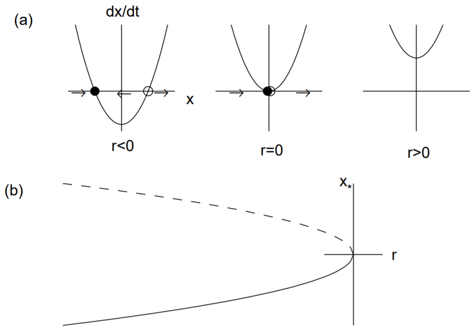
The saddle-node bifurcation results in fixed points being created or destroyed. The normal form for a saddle-node bifurcation is given by
\[\dot{x}=r+x^{2} . \nonumber \]
The fixed points are \(x_{*}=\pm \sqrt{-r}\). Clearly, two real fixed points exist when \(r<0\) and no real fixed points exist when \(r>0\). The stability of the fixed points when \(r<0\) are determined by the derivative of \(f(x)=r+x^{2}\), given by \(f^{\prime}(x)=2 x .\) Therefore, the negative fixed point is stable and the positive fixed point is unstable.

We can illustrate this bifurcation. First, in Fig. 12.1(a), we plot \(\dot{x}\) versus \(x\) for the three parameter values corresponding to \(r<0, r=0\) and \(r>0\). The values at which \(\dot{x}=0\) correspond to the fixed points, and arrows are drawn indicating how the solution \(x(t)\) evolves (to the right if \(\dot{x}>0\) and to the left if \(\dot{x}<0\) ). The stable fixed point is indicated by a filled circle and the unstable fixed point by an open circle. Note that when \(r=0\), solutions converge to the origin from the left, but diverge from the origin on the right.
Second, we plot the standard bifurcation diagram in Fig. 12.1(b), where the fixed point \(x_{*}\) is plotted versus the bifurcation parameter \(r\). As is the custom, the stable fixed point is denoted by a solid line and the unstable fixed point by a dashed line. Note that the two fixed points collide and annihilate at \(r=0\), and there are no fixed points for \(r>0\).
Transcritical bifurcation
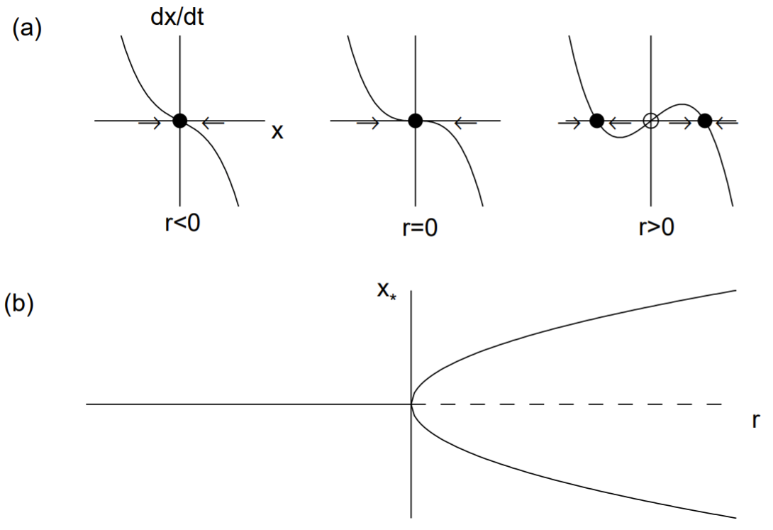
A transcritical bifurcation occurs when there is an exchange of stabilities between two fixed points. The normal form for a transcritical bifurcation is given by
\[\dot{x}=r x-x^{2} . \nonumber \]
The fixed points are \(x_{*}=0\) and \(x_{*}=r\). The derivative of the right-hand-side is \(f^{\prime}(x)=r-2 x\), so that \(f^{\prime}(0)=r\) and \(f^{\prime}(r)=-r\). Therefore, for \(r<0, x_{*}=0\) is stable and \(x_{*}=r\) is unstable, while for \(r>0, x_{*}=r\) is stable and \(x_{*}=0\) is unstable. The two fixed points thus exchange stability as \(r\) passes through zero. The transcritical bifurcation is illustrated in Fig. 12.2.
Pitchfork bifurcations
The pitchfork bifurcations occur when one fixed point becomes three at the bifurcation point Pitchfork bifurcations are usually associated with the physical phenomena called symmetry breaking. Pitchfork bifurcations come in two types. In the supercritical pitchfork bifurcation, the stability of the original fixed point changes from stable to unstable and a new pair of stable fixed points are created above (super-) the bifurcation point. In the subcritical bifurcation, the stability of the original fixed point again changes from stable to unstable but a new pair of now unstable fixed points are created below (sub-) the bifurcation point.
Supercritical pitchfork bifurcation
The normal form for the supercritical pitchfork bifurcation is given by
\[\dot{x}=r x-x^{3} \nonumber \]
Note that the linear term results in exponential growth when \(r>0\) and the nonlinear term stabilizes this growth. The fixed points are \(x_{*}=0\) and \(x_{*}=\pm \sqrt{r}\), the latter fixed points existing only when \(r>0\). The derivative of \(f\) is \(f^{\prime}(x)=r-3 x^{2}\) so that \(f^{\prime}(0)=r\) and \(f^{\prime}(\pm \sqrt{r})=-2 r\). Therefore, the fixed point \(x_{*}=0\) is stable for \(r<0\) and unstable for \(r>0\) while the fixed points \(x=\pm \sqrt{r}\) exist and are stable for \(r>0 .\) Notice that the fixed point \(x_{*}=0\) becomes unstable as \(r\) crosses zero and two new stable fixed points \(x_{*}=\pm \sqrt{r}\) are born. The supercritical pitchfork bifurcation is illustrated in Fig. 12.3.
The pitchfork bifurcation illustrates the physics of symmetry breaking. The differential equation (12.12) is invariant under the transformation \(x \rightarrow-x\). Fixed point solutions of this equation that obey this same symmetry are called symmetric; fixed points that do not are called asymmetric. Here, \(x_{*}=0\) is the symmetric fixed point and \(x=\pm \sqrt{r}\) are asymmetric. Asymmetric fixed points always occur in pairs, and mirror each others stability characteristics. Only the initial conditions determine which asymmetric fixed point is asymptotically attained.
Subcritical pitchfork bifurcation
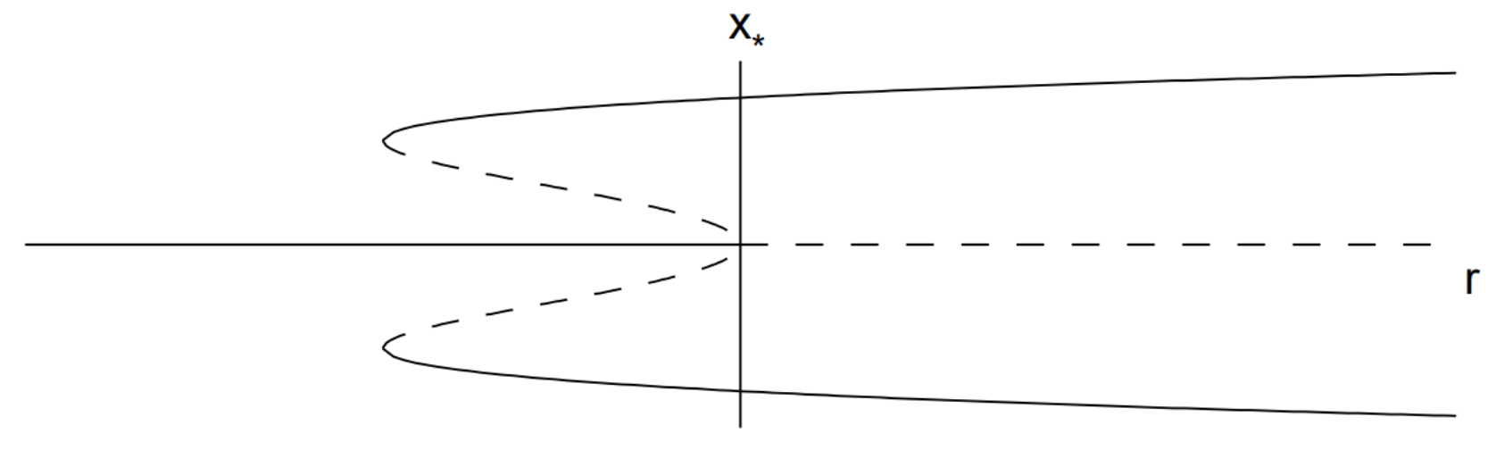
In the subcritical case, the cubic term is destabilizing. The normal form (to order \(x^{3}\) ) is
\[\dot{x}=r x+x^{3} \nonumber \]
The fixed points are \(x_{*}=0\) and \(x_{*}=\pm \sqrt{-r}\), the latter fixed points existing only when \(r \leq 0\). The derivative of the right-hand-side is \(f^{\prime}(x)=r+3 x^{2}\) so that \(f^{\prime}(0)=r\) and \(f^{\prime}(\pm \sqrt{-r})=-2 r .\) Therefore, the fixed point \(x_{*}=0\) is stable for \(r<0\) and unstable for \(r>0\) while the fixed points \(x=\pm \sqrt{-r}\) exist and are unstable for \(r<0\). There are no stable fixed points when \(r>0\).
The absence of stable fixed points for \(r>0\) indicates that the neglect of terms of higher-order in \(x\) than \(x^{3}\) in the normal form may be unwarranted. Keeping to the intrinsic symmetry of the equations (only odd powers of \(x\) so that the equation is invariant when \(x \rightarrow-x\) ) we can add a stabilizing nonlinear term proportional to \(x^{5}\). The extended normal form (to order \(x^{5}\) ) is
\[\dot{x}=r x+x^{3}-x^{5}, \nonumber \]
and is somewhat more difficult to analyze. The fixed points are solutions of
\[x\left(r+x^{2}-x^{4}\right)=0 . \nonumber \]
The fixed point \(x_{*}=0\) exists for all \(r\), and four additional fixed points can be found from the solutions of the quadratic equation in \(x^{2}\) :
\[x_{*}=\pm \sqrt{\frac{1}{2}(1 \pm \sqrt{1+4 r})} . \nonumber \]
These fixed points exist only if \(x_{*}\) is real. Clearly, for the inner square-root to be real, \(r \geq-1 / 4\). Also observe that \(1-\sqrt{1+4 r}\) becomes negative for \(r>0\). We thus have three intervals in \(r\) to consider, and these regions and their fixed points are
\[\begin{aligned} r<-\frac{1}{4}: & x_{*}=0 \quad \text { (one fixed point); } \\ -\frac{1}{4}<r<0: & x_{*}=0, \quad x_{*}=\pm \sqrt{\frac{1}{2}(1 \pm \sqrt{1+4 r})} \quad \text { (five fixed points); } \\ r>0: \quad x_{*}=0, \quad x_{*}=\pm \sqrt{\frac{1}{2}(1+\sqrt{1+4 r})} \quad \text { (three fixed points). } \end{aligned} \nonumber \]
Stability is determined from \(f^{\prime}(x)=r+3 x^{2}-5 x^{4} .\) Now, \(f^{\prime}(0)=r\) so \(x_{*}=0\) is stable for \(r<0\) and unstable for \(r>0\). The calculation for the other four roots can be simplified by noting that \(x_{*}\) satisfies \(r+x_{*}^{2}-x_{*}^{4}=0\), or \(x_{*}^{4}=r+x_{*}^{2} .\) Therefore,
\[\begin{aligned} f^{\prime}\left(x_{*}\right) &=r+3 x_{*}^{2}-5 x_{*}^{4} \\ &=r+3 x_{*}^{2}-5\left(r+x_{*}^{2}\right) \\ &=-4 r-2 x_{*}^{2} \\ &=-2\left(2 r+x_{*}^{2}\right) \end{aligned} \nonumber \]
With \(x_{*}^{2}=\frac{1}{2}(1 \pm \sqrt{1+4 r})\), we have
\[\begin{aligned} f^{\prime}\left(x_{*}\right) &=-2\left(2 r+\frac{1}{2}(1 \pm \sqrt{1+4 r})\right) \\ &=-((1+4 r) \pm \sqrt{1+4 r}) \\ &=-\sqrt{1+4 r}(\sqrt{1+4 r} \pm 1) \end{aligned} \nonumber \]
Clearly, the plus root is always stable since \(f^{\prime}\left(x_{*}\right)<0 .\) The minus root exists only for \(-\frac{1}{4}<r<0\) and is unstable since \(f^{\prime}\left(x_{*}\right)>0 .\) We summarize the stability of the various fixed points:
\[\begin{aligned} r<-\frac{1}{4}: \quad x_{*} &=0 \quad(\text { stable }) ; \\ -\frac{1}{4}<r<0: \quad x_{*} &=0, \quad(\text { stable }) \\ x_{*} &=\pm \sqrt{\frac{1}{2}(1+\sqrt{1+4 r})} \quad \text { (stable); } \\ x>0: \quad x_{*} &=\pm \sqrt{\frac{1}{2}(1-\sqrt{1+4 r})} \quad \text { (unstable); } \\ x_{*} &=0 \quad(\text { unstable }) \\ x_{*} &=\pm \sqrt{\frac{1}{2}(1+\sqrt{1+4 r})} \quad \text { (stable). } \end{aligned} \nonumber \]
The bifurcation diagram is shown in Fig. 12.4. Notice that there in addition to a subcritical pitchfork bifurcation at the origin, there are two symmetric saddlenode bifurcations that occur when \(r=-1 / 4\).
We can imagine what happens to the solution to the ode as \(r\) increases from negative values, supposing there is some noise in the system so that \(x(t)\) fluctuates around a stable fixed point. For \(r<-1 / 4\), the solution \(x(t)\) fluctuates around the stable fixed point \(x_{*}=0\). As \(r\) increases into the range \(-1 / 4<r<0\), the solution will remain close to the stable fixed point \(x_{*}=0 .\) However, a so-called catastrophe occurs as soon as \(r>0 .\) The \(x_{*}=0\) fixed point is lost and the solution will jump up (or down) to the only remaining fixed point. A similar catastrophe can happen as \(r\) decreases from positive values. In this case, the jump occurs as soon as \(r<-1 / 4\). Since the behavior of \(x(t)\) is different depending on whether we increase or decrease \(r\), we say that the system exhibits hysteresis. The existence of a subcritical pitchfork bifurcation can be very dangerous in engineering applications since a small change in the physical parameters of a problem can result in a large change in the equilibrium state. Physically, this can result in the collapse of a structure.
Hopf bifurcations
A new type of bifurcation can occur in two dimensions. Suppose there is some control parameter \(\mu\). Furthermore, suppose that for \(\mu<0\), a two-dimensional system approaches a fixed point by exponentially-damped oscillations. We know that the Jacobian matrix at the fixed point with \(\mu<0\) will have complex conjugate eigenvalues with negative real parts. Now suppose that when \(\mu>0\) the real parts of the eigenvalues become positive so that the fixed point becomes unstable. This change in stability of the fixed point is called a Hopf bifurcation. The Hopf bifurcations also come in two types: a supercritical Hopf bifurcation and a subcritical Hopf bifurcation. For the supercritical Hopf bifurcation, as \(\mu\) increases slightly above zero, the resulting oscillation around the now unstable fixed point is quickly stabilized at small amplitude, and one obtains a limit cycle. For the subcritical Hopf bifurcation, as \(\mu\) increases slightly above zero, the limit cycle immediately jumps to large amplitude.
Phase portraits
The phase space of a dynamical system consists of the independent dynamical variables. For example, the phase space of the damped, driven pendulum equations given by (11.15) is three dimensional and consists of \(\theta, u\) and \(\phi\). The unforced equations have only a two-dimensional phase space, consisting of \(\theta\) and \(u\).
An important feature of paths in phase space is that they can never cross except at a fixed point, which may be stable if all paths go into the point, or unstable if some paths go out. This is a consequence of the uniqueness of the solution to a differential equation. Every point on the phase-space diagram represents a possible initial condition for the equations, and must have a unique trajectory associated with that initial condition.
The simple pendulum is a conservative system, exhibiting a conservation law for energy, and this implies a conservation of phase space area (or volume). The damped pendulum is nonconservative, however, and this implies a shrinking of phase space area (or volume).
Indeed, it is possible to derive a general condition to determine whether phase space volume is conserved or shrinks. We consider here, for convenience, equations in a three-dimensional phase space given by
\[\dot{x}=F(x, y, z), \quad \dot{y}=G(x, y, z), \quad \dot{z}=H(x, y, z) . \nonumber \]
We can consider a small volume of phase space \(\Gamma=\Gamma(t)\), given by
\[\Gamma(t)=\Delta x \Delta y \Delta z, \nonumber \]
where
\[\Delta x=x_{1}(t)-x_{0}(t), \quad \Delta y=y_{1}(t)-y_{0}(t), \quad \Delta z=z_{1}(t)-z_{0}(t) \nonumber \]
The initial phase-space volume at time \(t\) represents a box with one corner at the point \(\left(x_{0}(t), y_{0}(t), z_{0}(t)\right)\) and the opposing corner at \(\left(x_{1}(t), y_{1}(t), z_{1}(t)\right)\). This initial phase-space box then evolves over time. To determine how an edge emanating from \(\left(x_{0}, y_{0}, z_{0}\right)\) with length \(\Delta x\) evolves, we write using a first-order Taylor series expansion in \(\Delta t\)
\[\begin{aligned} &x_{0}(t+\Delta t)=x_{0}(t)+\Delta t F\left(x_{0}, y_{0}, z_{0}\right) \\ &x_{1}(t+\Delta t)=x_{1}(t)+\Delta t F\left(x_{1}, y_{0}, z_{0}\right) \end{aligned} \nonumber \]
Therefore,
\[\Delta x(t+\Delta t)=\Delta x(t)+\Delta t\left(F\left(x_{1}, y_{0}, z_{0}\right)-F\left(x_{0}, y_{0}, z_{0}\right)\right) \nonumber \]
Subtracting \(\Delta x(t)\) from both sides and dividing by \(\Delta t\), we have as \(\Delta t \rightarrow 0\),
\[\frac{d}{d t}(\Delta x)=\left(F\left(x_{1}, y_{0}, z_{0}\right)-F\left(x_{0}, y_{0}, z_{0}\right)\right) . \nonumber \]
With \(\Delta x\) small, we therefore obtain to first order in \(\Delta x\),
\[\frac{d}{d t}(\Delta x)=\Delta x \frac{\partial F}{\partial x}, \nonumber \]
where the partial derivative is evaluated at the point \(\left(x_{0}(t), y_{0}(t), z_{0}(t)\right)\).
Similarly, we also have
\[\frac{d}{d t}(\Delta y)=\Delta y \frac{\partial G}{\partial y}, \quad \frac{d}{d t}(\Delta z)=\Delta z \frac{\partial H}{\partial z} \nonumber \]
Since
\[\frac{d \Gamma}{d t}=\frac{d(\Delta x)}{d t} \Delta y \Delta z+\Delta x \frac{d(\Delta y)}{d t} \Delta z+\Delta x \Delta y \frac{d(\Delta z)}{d t} \nonumber \]
we have
\[\frac{d \Gamma}{d t}=\left(\frac{\partial F}{\partial x}+\frac{\partial G}{\partial y}+\frac{\partial H}{\partial z}\right) \Gamma \nonumber \]
valid for the evolution of an infinitesimal box.
We can conclude from (12.25) that phase-space volume is conserved if the divergence on the right-hand-side vanishes, or that phase-space volume contracts exponentially if the divergence is negative.
For example, we can consider the equations for the damped, driven pendulum given by (11.15). The divergence in this case is derived from
\[\frac{\partial}{\partial \theta}(u)+\frac{\partial}{\partial u}\left(-\frac{1}{q} u-\sin \theta+f \cos \psi\right)+\frac{\partial}{\partial \psi}(\omega)=-\frac{1}{q} \nonumber \]
and provided \(q>0\) (i.e., the pendulum is damped), phase-space volume contracts. For the undamped pendulum (where \(q \rightarrow \infty\) ), phase-space volume is conserved.
Limit cycles
The asymptotic state of a nonlinear system may be a limit cycle instead of a fixed point. A stable limit cycle is a periodic solution on which all nearby solutions converge. Limit cycles can also be unstable. Determining the existence of a limit cycle from a nonlinear system of equations through analytical means is usually impossible, but limit cycles are easily found numerically. The damped, driven pendulum equations has no fixed points, but does have limit cycles.
Attractors and basins of attraction
An attractor is a stable configuration in phase space. For example, an attractor can be a stable fixed point or a limit cycle. The damped, non-driven pendulum converges to a stable fixed point corresponding to the pendulum at rest at the bottom. The damped, driven pendulum for certain values of the parameters converges to a limit cycle. We will see that the chaotic pendulum also has an attractor of a different sort, called a strange attractor.
The domain of attraction of a stable fixed point, or of a limit cycle, is called the attractor’s basin of attraction. The basin of attraction consists of all initial conditions for which solutions asymptotically converge to the attractor. For nonlinear systems, basins of attraction can have complicated geometries.
Poincaré sections
The Poincaré section is a method to reduce by one or more dimensions the phase space diagrams of higher dimensional systems. Most commonly, a three-dimensional phase space can be reduced to two-dimensions, for which a plot may be easier to interpret. For systems with a periodic driving force such as the damped, driven pendulum system given by (11.15), the two-dimensional phase space \((\theta, u)\) can be viewed stroboscopically, with the strobe period taken to be the period of forcing, that is \(2 \pi / \omega\). For the damped, driven pendulum, the third dynamical variable \(\psi\) satisfies \(\psi=\psi_{0}+\omega t\), and the plotting of the phase-space variables \((\theta, u)\) at the times \(t_{0}, t_{0}+2 \pi / \omega\), \(t_{0}+4 \pi / \omega\), etc., is equivalent to plotting the values of \((\theta, u)\) every time the phase-space variable \(\psi\) in incremented by \(2 \pi\).
For systems without periodic forcing, a plane can be placed in the three-dimensional phase space, and a point can be plotted on this plane every time the orbit passes through it. For example, if the dynamical variables are \(x, y\) and \(z\), a plane might be placed at \(z=0\) and the values of \((x, y)\) plotted every time z passes through zero. Usually, one also specifies the direction of passage, so that a point is plotted only when \(\dot{z}>0\), say.
Fractal dimensions
The attractor of the chaotic pendulum is called strange because it occupies a fractional dimension of phase space. To understand what is meant by fractional dimensions, we first review some classical fractals.
Classical fractals
Cantor set

The Cantor set has some unusual properties. First, we compute its length. Let \(l_{n}\) denote the length of the set \(S_{n} .\) Clearly, \(l_{0}=1 .\) Since \(S_{1}\) is constructed by removing the middle third of \(S_{0}\), we have \(l_{1}=2 / 3\). To construct \(S_{2}\), we again remove the middle third of the two line segments of \(S_{1}\), reducing the length of \(S_{1}\) by another factor of \(2 / 3\), so that \(l_{2}=(2 / 3)^{2}\), and so on. We obtain \(l_{n}=(2 / 3)^{n}\), and the \(\lim _{n \rightarrow \infty} l_{n}=0 .\) Therefore, the Cantor set has zero length.
The Cantor set, then, does not consist of line segments. Yet, the Cantor set is certainly not an empty set. We can see that at stage 1 , there are two interior endpoints \(1 / 3\) and \(2 / 3\), and these will never be removed; at stage 2 , there are the additional interior endpoints \(1 / 9,2 / 9,7 / 9\) and \(8 / 9\); and at stage 3 , we add eight more interior endpoints. We see, then, that at stage \(k\) we add \(2^{k}\) more interior endpoints. An infinite but countable number of endpoints are therefore included in the Cantor set.
But the Cantor set consists of much more than just these endpoints, and we will in fact show that the Cantor set is an uncountable set. Recall from analysis, that an infinite set of points can be either countable or uncountable. A countable set of points is a set that can be put in a oneto-one correspondence with the set of natural numbers. As is well known, the infinite set of all rational numbers is countable whereas the infinite set of real numbers is uncountable. By listing the endpoints of the Cantor set above, each stage adding \(2^{k}\) more endpoints, we have shown that the set of all endpoints is a countable set.
In order to prove that the Cantor set is uncountable, it is helpful to make use of the base 3 representation of numbers. Recall that any number \(N\), given by
\[N=\ldots \mathrm{a} * B^{3}+\mathrm{b} * B^{2}+\mathrm{c} * B+\mathrm{d} * B^{0}+\mathrm{e} * B^{-1}+\mathrm{f} * B^{-2}+\mathrm{g} * B^{-3}+\ldots, \nonumber \]
can be written in base \(B\) as
\[N=\ldots \text { abcd.efg } \ldots \text { (base } B \text { ) } \nonumber \]
where the period separating the integer part of the number from the fractional part is in general called a radix point. For base 10, of course, the radix point is called a decimal point, and for base 2, a binary point.
Now, consider the Cantor set. In the first stage, all numbers lying between \(1 / 3\) and \(2 / 3\) are removed. The remaining numbers, then, must be of the form \(0.0 \ldots\) (base 3 ) or \(0.2 \ldots\) (base 3 ), since (almost) all the numbers having the form \(0.1 \ldots\) (base 3) have been removed. The single exception is the endpoint \(1 / 3=0.1\) (base 3 ), but this number can also be written as \(1 / 3=0.02\) (base 3 ), where the bar over a number or numbers signifies an infinite repetition. In the second stage, all numbers lying between \(1 / 9\) and \(2 / 9\), say, are removed, and these numbers are of the form \(0.01 \ldots\) (base 3). We can see, then, that the Cantor set can be defined as the set of all numbers on the unit interval that contain no 1’s in their base 3 representation.
Using base 3 notation, it is easy to find a number that is not an endpoint, yet is in the Cantor set. For example, the number \(1 / 4\) is not an endpoint. We can convert \(1 / 4\) to base 3 by the following calculation:
\[\begin{aligned} \frac{1}{4} \times 3 &=0.75 \\ 0.75 \times 3 &=2.25 \\ 0.25 \times 3 &=0.75 \\ 0.75 \times 3 &=2.25 \end{aligned} \nonumber \]
and so on, from which we find that \(1 / 4=0 . \overline{02}\) (base 3 ). The number \(1 / 4\), therefore, has no 1 ’s in its base 3 expansion and so is an element of the Cantor set.
We can now prove that the Cantor set is an uncountable set. The proof is similar to that used to prove that the real numbers are uncountable. If we suppose that the Cantor set is countable, then we can list all of its elements using a base 3 expansion; that is,
\[\begin{aligned} &x_{1}=0 . x_{11} x_{12} x_{13} \ldots(\text { base } 3), \\ &x_{2}=0 . x_{21} x_{22} x_{23} \ldots(\text { base } 3), \\ &x_{3}=0 . x_{31} x_{32} x_{33} \ldots(\text { base } 3), \end{aligned} \nonumber \]
and so on, where all the \(x_{i j}\) ’s must be either a 0 or a 2 (i.e., no 1 ’s are allowed). It is now simple to name a number \(y\) not on this list. We have
\[y=0 . y_{11} y_{22} y_{33} \cdots \nonumber \]
where \(y_{11} \neq x_{11}, y_{22} \neq x_{22}, y_{33} \neq x_{33}\), etc.. That is, if \(x_{11}=0\), then \(y_{11}=2 ;\) if \(x_{11}=2\), then \(y_{11}=0\), and so on. By constructing a number not on the list, we have obtained a reductio ad absurdum, and we can conclude that the Cantor set is uncountable.
Note that the endpoints of the Cantor set are just those numbers written in base 3 that end with either all 0 ’s or all 2 ’s, and these indeed form only a very small subset of the entire Cantor set.
From the base 3 representation, we can now see that the Cantor set has the following interesting characteristic. On the one hand, any small interval around a point in the Cantor set contains another point in the Cantor set. On the other hand, there is an interval between any two points in the Cantor set that is not in the Cantor set. For example, take the point \(1 / 4=0 . \overline{02}\) in the Cantor set, and the interval \(\left[1 / 4-3^{-4}, 1 / 4+3^{-4}\right] .\) In base 3 , the interval is given by \([0.0201 \overline{02}, 0.0210 \overline{02}]\). There are, of course, an infinite number of points in the Cantor set in this interval, one of them being \(0.0202\) to the left of \(1 / 4\), and \(0.02022\) to the right of \(1 / 4\). If the interval was established using \(3^{-n}\), for any \(n\), we can still find other points in the interval that are in the Cantor set. Also, between any two points in the Cantor set, there is an interval that was removed during the construction of the Cantor set. So the Cantor set consists of neither line segments nor a set of discrete points.
The Cantor set is also self-similar, meaning that it contains smaller copies of itself at all scales.
The Cantor set is called a fractal, and is said to have a fractal dimension. Integer dimensions are more familiar to us: we say that a line has dimension 1 ; an area, dimension 2 ; and a volume, dimension \(3 .\)
For self-similar sets, we can place the definition of dimension on a more mathematical basis. A line segment, a square, and a cube can also be considered self-similar. Suppose that a selfsimilar set \(S\) is composed of \(m\) copies of itself scaled down by a factor of \(r\). As examples, the line segment \([0,1]\) is composed of two copies of itself scaled down by a factor of two; namely, the segments \([0,1 / 2]\) and \([1 / 2,1]\). A square is composed of four copies of itself scaled down by a factor of two. And a cube is composed of eight copies of itself scaled down by a factor of two. We write
\[m=r^{D}, \nonumber \]
where \(D\) is called the similarity dimension of the set. With \(r=2\), the line segment has \(m=2\), the square has \(m=4\), and the cube has \(m=8\), yielding the usual dimensions \(D=1,2\) and 3 , respectively.
Now the Cantor set is composed of two copies of itself scaled down by a factor of three. Therefore,
\[2=3^{D}, \nonumber \]
and the similarity dimension of the Cantor set is given by \(D=\log 2 / \log 3 \approx 0.6309\), which has dimension smaller than that of a line, but larger than that of a point.
Sierpinski triangle
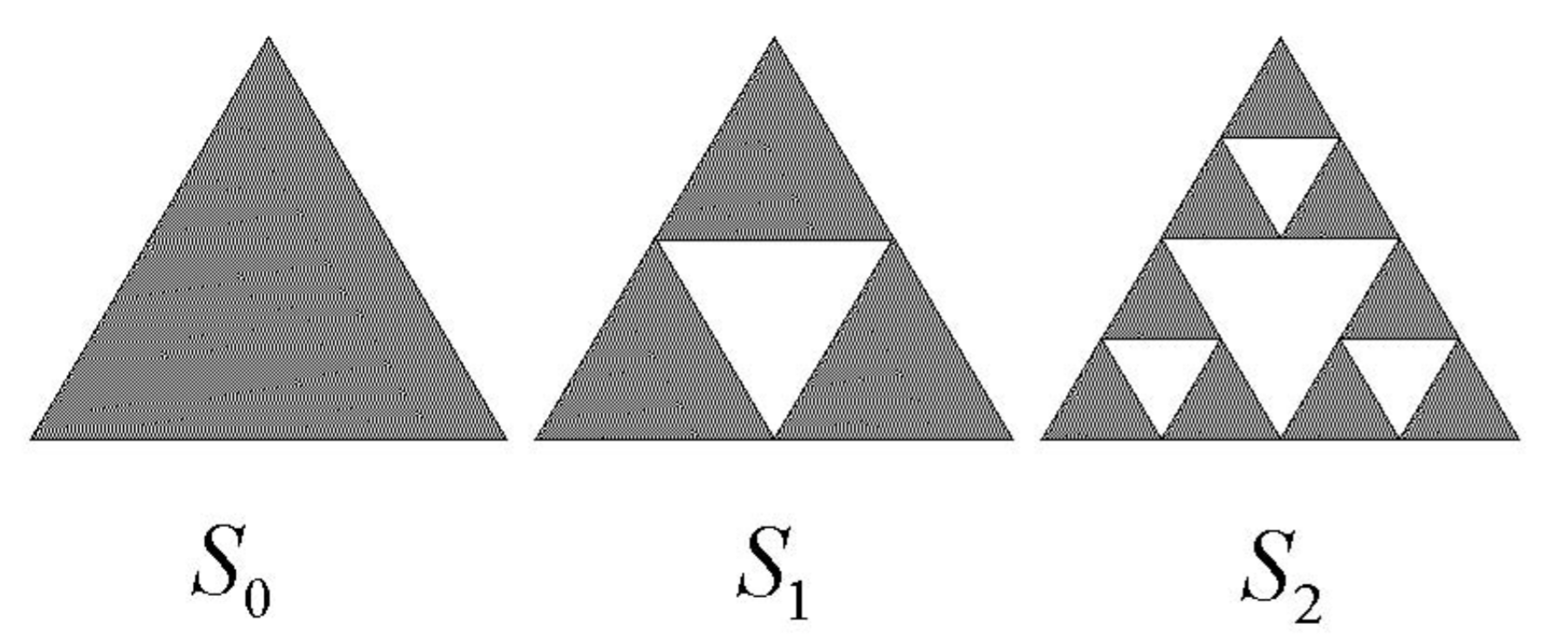
Other classical fractals can be constructed similarly to the Cantor set. The Sierpinski triangle starts with an equilateral triangle, \(S_{0}\), with unit sides. We then draw lines connecting the three midpoints of the three sides. The just formed equilateral middle triangle of side length \(1 / 2\) is then removed from \(S_{0}\) to form the set \(S_{1}\). This process is repeated on the remaining equilateral triangles, as illustrated in Fig. 12.6. The Sierpinski triangle \(S\) is defined as the limit of this repetition; that is, \(S=\lim _{n \rightarrow \infty} S_{n}\).
The Sierpinski triangle is composed of three copies of itself scaled down by a factor of two, so that
\[3=2^{D}, \nonumber \]
and the similarity dimension is \(D=\log 3 / \log 2 \approx 1.5850\), which has dimension between a line and an area.
Similar to the Cantor set, the Sierpinksi triangle, though existing in a two-dimensional space, has zero area. If we let \(A_{i}\) be the area of the set \(S_{i}\), then since area is reduced by a factor of \(3 / 4\) with each iteration, we have
\[A_{n}=\left(\frac{3}{4}\right)^{n} A_{0} \nonumber \]
so that \(A=\lim _{n \rightarrow \infty} A_{n}=0\).
Sierpinski carpet
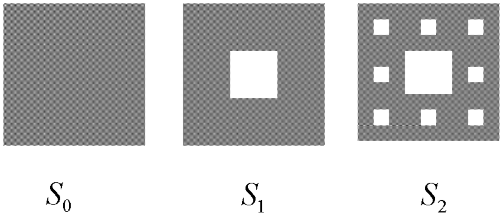
The Sierpinski carpet starts with a square, \(S_{0, \text { with unit sides. Here, we remove a center }}\) square of side length \(1 / 3\); the remaining set is called \(S_{1}\). This process is then repeated as illustrated in Fig. 12.7.
Here, the Sierpinski carpet is composed of eight copies of itself scaled down by a factor of three, so that
\[8=3^{D} \text {, } \nonumber \]
and the similarity dimension is \(D=\log 8 / \log 3 \approx 1.8928\), somewhat larger than the Sierpinski triangle. One can say, then, that the Sierpinski carpet is more space filling than the Sierpinski triangle, though it still has zero area.
Koch curve
Like the Cantor set, we start with the unit interval, but now we replace the middle one-third by two line segments of length \(1 / 3\), as illustrated in \(12.8\), to form the set \(S_{1}\). This process is then repeated on the four line segments of length \(1 / 3\) to form \(S_{2}\), and so on, as illustrated in Fig. \(12.8\).
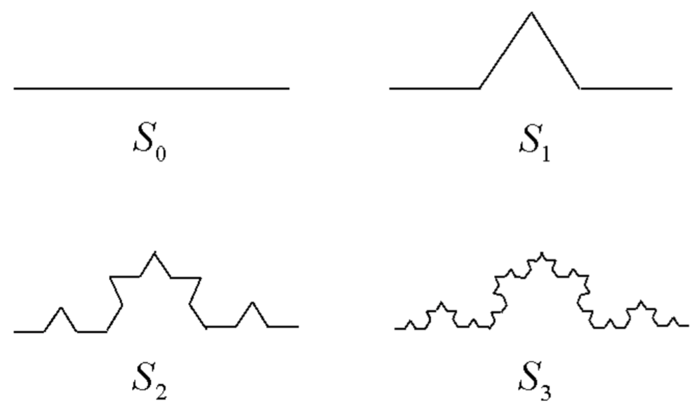
Here, the Koch curve is composed of four copies of itself scaled down by a factor of three, so that
\[4=3^{D} \nonumber \]
and the similarity dimension is \(D=\log 4 / \log 3 \approx 1.2619 .\) The Koch curve therefore has a dimension lying between a line and an area. Indeed, with each iteration, the length of the Koch curve increases by a factor of \(4 / 3\) so that its length is infinite.
Koch snow flake
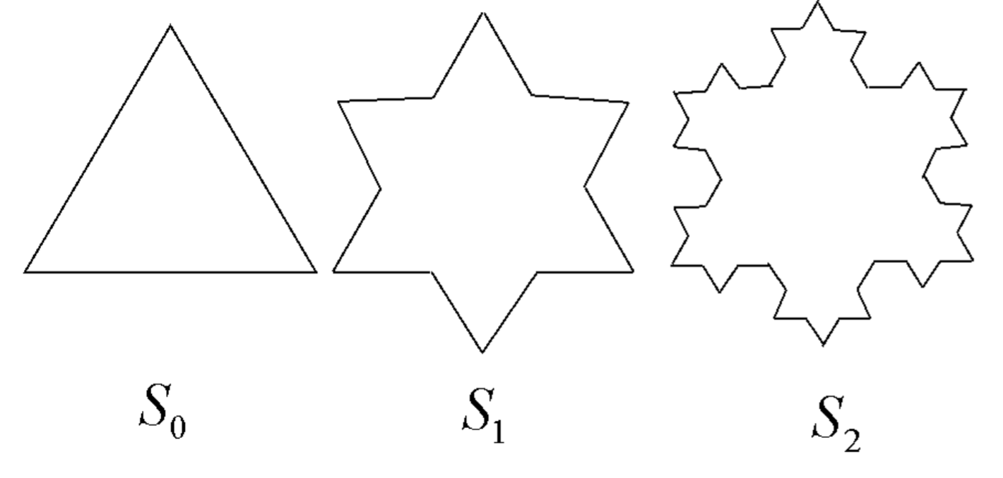
Here, we start with an equilateral triangle. Similar to the Koch curve, we replace the middle one-third of each side by two line segments, as illustrated in 12.9. The boundary of the Koch snow flake has the same fractal dimension as the Koch curve, and is of infinite length. The area bounded by the boundary is obviously finite, however, and can be shown to be \(8 / 5\) of the area of the original triangle. Interestingly, here an infinite perimeter encloses a finite area.
Correlation Dimension
Modern studies of dynamical systems have discovered sets named strange attractors. These sets share some of the characteristics of classical fractals: they are not space filling yet have structure at arbitrarily small scale. However, they are not perfectly self-similar in the sense of the classical fractals, having arisen from the chaotic evolution of some dynamical system. Here, we attempt to generalize the definition of dimension so that it is applicable to strange attractors and relatively easy to compute. The definition and numerical algorithm described here was first proposed in a paper by Grassberger and Procaccia (1993)
Definitions
Consider a set \(S\) of \(N\) points. Denote the points in this set as \(\mathbf{x}_{i}\), with \(i=1,2, \ldots, N\) and denote the distance between two points \(\mathbf{x}_{i}\) and \(\mathbf{x}_{j}\) as \(r_{i j} .\) Note that there are \(N(N-1) / 2\) distinct distances. We define the correlation integral \(C(r)\) to be
\[C(r)=\lim _{N \rightarrow \infty} \frac{2}{N(N-1)} \times\left\{\text { number of distinct distances } r_{i j} \text { less than } r\right\} . \nonumber \]
If \(C(r) \propto r^{D}\) over a wide range of \(r\) when \(N\) is sufficiently large, then \(D\) is to be called the correlation dimension of the set \(S\). Note that with this normalization, \(C(r)=1\) for \(r\) larger than the largest possible distance between two points on the set \(S\).
The correlation dimension agrees with the similarity dimension for an exactly self-similar set. As a specific example, consider the Cantor set. Suppose \(N\) points that lie on the Cantor set are chosen at random to be in \(S\). Since every point on the set is within a distance \(r=1\) of every other point, one has \(C(1)=1\). Now, approximately one-half of the points in \(S\) lie between 0 and \(1 / 3\), and the other half lie between \(2 / 3\) and 1. Therefore, only 1/2 of the possible distinct distances \(r_{i j}\) will be less than \(1 / 3\) (as \(N \rightarrow \infty\) ), so that \(C(1 / 3)=1 / 2\). Continuing in this fashion, we find in general that \(C\left(1 / 3^{s}\right)=1 / 2^{s}\). With \(r=1 / 3^{s}\), we have
\[s=-\frac{\log r}{\log 3} \nonumber \]
so that
\[\begin{aligned} C(r) &=2^{\log r / \log 3} \\ &=\exp (\log 2 \log r / \log 3) \\ &=r^{\log 2 / \log 3}, \end{aligned} \nonumber \]
valid for small values of \(r .\) We have thus found a correlation dimension, \(D=\log 2 / \log 3\), in agreement with the previously determined similarity dimension.
Numerical computation
Given a finite set \(S\) of \(N\) points, we want to formulate a fast numerical algorithm to compute \(C(r)\) over a sufficiently wide range of \(r\) to accurately determine the correlation dimension \(D\) from a log-log plot of \(C(r)\) versus \(r .\) A point \(\mathbf{x}_{i}\) in the set \(S\) may be a real number, or may be a coordinate pair. If the points come from a Poincaré section, then the fractal dimension of the Poincaré section will be one less than the actual fractal dimension of the attractor in the full phase space.
Define the distance \(r_{i j}\) between two points \(\mathbf{x}_{i}\) and \(\mathbf{x}_{j}\) in \(S\) to be the standard Euclidean distance. To obtain an accurate value of \(D\), one needs to throw away an initial transient before collecting points for the set \(S\). Since we are interested in a graph of \(\log C\) versus \(\log r\), we compute \(C(r)\) at points \(r\) that are evenly spaced in \(\log r .\) For example, we can compute \(C(r)\) at the points \(r_{s}=2^{s}\), where \(s\) takes on integer values.
First, one counts the number of distinct distance \(r_{i j}\) that lie in the interval \(r_{s-1} \leq r_{i j}<r_{s}\). Denote this count by \(M(s)\). An approximation to the correlation integral \(C\left(r_{s}\right)\) using the \(N\) data points is then obtained from
\[C\left(r_{s}\right)=\frac{2}{N(N-1)} \sum_{s^{\prime}=-\infty}^{s} M\left(s^{\prime}\right) \nonumber \]
One can make use of a built-in MATLAB function to speed up the computation. The function call
![Matrix equation showing the commutator \([F, E]\) as equal to \(\log_2(x)\).](https://math.libretexts.org/@api/deki/files/77417/clipboard_ea9ff6253d7cc8730412cae9a9cbb5ae5.png?revision=1)
returns the floating point number \(\mathrm{F}\) and the integer \(\mathrm{E}\) such that \(\mathrm{x}=\mathrm{F} * 2^{\wedge} \mathrm{E}\), where \(0.5 \leq|\mathrm{F}|<1\) and \(\mathrm{E}\) is an integer. To count each \(r_{i j}\) in the appropriate bin \(M(s)\), one can compute all the values of \(r_{i j}\) and place them into the Matlab array \(r\). Then one uses the vector form of \(10 \mathrm{~g} 2 . \mathrm{m}\) to compute the corresponding values of \(s\) :
![Mathematical expression showing [~s] equals log base 2 of x.](https://math.libretexts.org/@api/deki/files/77418/clipboard_e87332d066a787e29c489c156c1c46927.png?revision=1&size=bestfit&width=295&height=30)
One can then increment the count in a Matlab array \(M\) that corresponds to the particular integer values of s. The Matlab function cumsum.m can then be used to compute the Matlab array C.
Finally, a least-squares analysis of the data is required to compute the fractal dimension \(D\). By directly viewing the log-log plot, one can choose which adjacent points to fit a straight line through, and then use the method of least-squares to compute the slope. The MATLAB function polyfit.m can determine the best fit line and the corresponding slope. Ideally, one would also compute a statistical error associated with this slope, and such an error should go to zero as the number of points computed approaches infinity.