
2.2: Bifurcation diagram for quadratic maps
- Page ID
- 101322
\( \newcommand{\vecs}[1]{\overset { \scriptstyle \rightharpoonup} {\mathbf{#1}} } \)
\( \newcommand{\vecd}[1]{\overset{-\!-\!\rightharpoonup}{\vphantom{a}\smash {#1}}} \)
\( \newcommand{\id}{\mathrm{id}}\) \( \newcommand{\Span}{\mathrm{span}}\)
( \newcommand{\kernel}{\mathrm{null}\,}\) \( \newcommand{\range}{\mathrm{range}\,}\)
\( \newcommand{\RealPart}{\mathrm{Re}}\) \( \newcommand{\ImaginaryPart}{\mathrm{Im}}\)
\( \newcommand{\Argument}{\mathrm{Arg}}\) \( \newcommand{\norm}[1]{\| #1 \|}\)
\( \newcommand{\inner}[2]{\langle #1, #2 \rangle}\)
\( \newcommand{\Span}{\mathrm{span}}\)
\( \newcommand{\id}{\mathrm{id}}\)
\( \newcommand{\Span}{\mathrm{span}}\)
\( \newcommand{\kernel}{\mathrm{null}\,}\)
\( \newcommand{\range}{\mathrm{range}\,}\)
\( \newcommand{\RealPart}{\mathrm{Re}}\)
\( \newcommand{\ImaginaryPart}{\mathrm{Im}}\)
\( \newcommand{\Argument}{\mathrm{Arg}}\)
\( \newcommand{\norm}[1]{\| #1 \|}\)
\( \newcommand{\inner}[2]{\langle #1, #2 \rangle}\)
\( \newcommand{\Span}{\mathrm{span}}\) \( \newcommand{\AA}{\unicode[.8,0]{x212B}}\)
\( \newcommand{\vectorA}[1]{\vec{#1}} % arrow\)
\( \newcommand{\vectorAt}[1]{\vec{\text{#1}}} % arrow\)
\( \newcommand{\vectorB}[1]{\overset { \scriptstyle \rightharpoonup} {\mathbf{#1}} } \)
\( \newcommand{\vectorC}[1]{\textbf{#1}} \)
\( \newcommand{\vectorD}[1]{\overrightarrow{#1}} \)
\( \newcommand{\vectorDt}[1]{\overrightarrow{\text{#1}}} \)
\( \newcommand{\vectE}[1]{\overset{-\!-\!\rightharpoonup}{\vphantom{a}\smash{\mathbf {#1}}}} \)
\( \newcommand{\vecs}[1]{\overset { \scriptstyle \rightharpoonup} {\mathbf{#1}} } \)
\( \newcommand{\vecd}[1]{\overset{-\!-\!\rightharpoonup}{\vphantom{a}\smash {#1}}} \)
There is a good way to trace bifurcations on the (x, c). Let us plot iterations fc: xo = 0 → x1 → x2 →...→ xMaxIt for all real c. Colors (from blue to red) show how often an orbit visits the pixel. You can watch iterations of fc(x) for corresponding c values on the right.

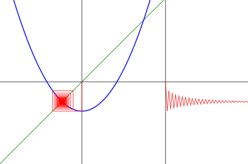
Controls: Click mouse to zoom in 2 times. Click mouse with Ctrl to zoom out. Hold Shift key to zoom in the c (vertical) direction only. Max number of iterations = 2000. See coordinates of the image center and Δx, Δc in the text field. The vertical line goes through x = 0.

The top part of the picture corresponds to a single attracting fixed point of f for -3/4 < c < 1/4. For c > 1/4 points go away to +∞ (see tangent bifurcation). Filaments and broadening show how the critical orbit points are attracted to the fixed point. Near c = -3/4 we see a branching point due to period doubling bifurcation. Then all the Feigenbaum's bifurcation cascade. At the lower part of the bifurcation diagram you see chaotic bands and white narrow holes of windows of periodic dynamics. The lowest and biggest one corresponds to the period-3 window.

Compare the map with the Mandelbrot set to the right.
The bifurcation map patterns
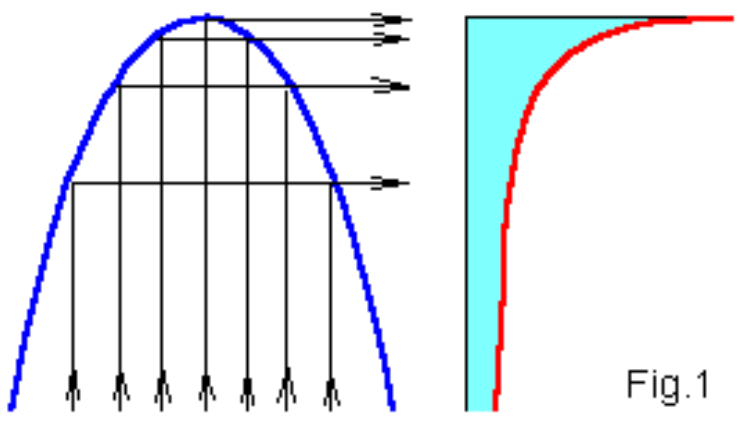
Fig.1 shows that caustics in distribution of points of chaotic orbits are generated by an extremum of a mapping. Therefore singularities (painted in the red) on the bifurcation diagram appear at images of the critical point fc on(0). Let us denote gn(c) = fcon(0), then
go(c) = 0, g1(c) = c, g2(c) = c2 + c, ...
The curves g0,1,...,6(c) are shown in Fig.2.
