1.6.6.5: Answers to exercises
- Page ID
- 32645
\( \newcommand{\vecs}[1]{\overset { \scriptstyle \rightharpoonup} {\mathbf{#1}} } \)
\( \newcommand{\vecd}[1]{\overset{-\!-\!\rightharpoonup}{\vphantom{a}\smash {#1}}} \)
\( \newcommand{\dsum}{\displaystyle\sum\limits} \)
\( \newcommand{\dint}{\displaystyle\int\limits} \)
\( \newcommand{\dlim}{\displaystyle\lim\limits} \)
\( \newcommand{\id}{\mathrm{id}}\) \( \newcommand{\Span}{\mathrm{span}}\)
( \newcommand{\kernel}{\mathrm{null}\,}\) \( \newcommand{\range}{\mathrm{range}\,}\)
\( \newcommand{\RealPart}{\mathrm{Re}}\) \( \newcommand{\ImaginaryPart}{\mathrm{Im}}\)
\( \newcommand{\Argument}{\mathrm{Arg}}\) \( \newcommand{\norm}[1]{\| #1 \|}\)
\( \newcommand{\inner}[2]{\langle #1, #2 \rangle}\)
\( \newcommand{\Span}{\mathrm{span}}\)
\( \newcommand{\id}{\mathrm{id}}\)
\( \newcommand{\Span}{\mathrm{span}}\)
\( \newcommand{\kernel}{\mathrm{null}\,}\)
\( \newcommand{\range}{\mathrm{range}\,}\)
\( \newcommand{\RealPart}{\mathrm{Re}}\)
\( \newcommand{\ImaginaryPart}{\mathrm{Im}}\)
\( \newcommand{\Argument}{\mathrm{Arg}}\)
\( \newcommand{\norm}[1]{\| #1 \|}\)
\( \newcommand{\inner}[2]{\langle #1, #2 \rangle}\)
\( \newcommand{\Span}{\mathrm{span}}\) \( \newcommand{\AA}{\unicode[.8,0]{x212B}}\)
\( \newcommand{\vectorA}[1]{\vec{#1}} % arrow\)
\( \newcommand{\vectorAt}[1]{\vec{\text{#1}}} % arrow\)
\( \newcommand{\vectorB}[1]{\overset { \scriptstyle \rightharpoonup} {\mathbf{#1}} } \)
\( \newcommand{\vectorC}[1]{\textbf{#1}} \)
\( \newcommand{\vectorD}[1]{\overrightarrow{#1}} \)
\( \newcommand{\vectorDt}[1]{\overrightarrow{\text{#1}}} \)
\( \newcommand{\vectE}[1]{\overset{-\!-\!\rightharpoonup}{\vphantom{a}\smash{\mathbf {#1}}}} \)
\( \newcommand{\vecs}[1]{\overset { \scriptstyle \rightharpoonup} {\mathbf{#1}} } \)
\(\newcommand{\longvect}{\overrightarrow}\)
\( \newcommand{\vecd}[1]{\overset{-\!-\!\rightharpoonup}{\vphantom{a}\smash {#1}}} \)
\(\newcommand{\avec}{\mathbf a}\) \(\newcommand{\bvec}{\mathbf b}\) \(\newcommand{\cvec}{\mathbf c}\) \(\newcommand{\dvec}{\mathbf d}\) \(\newcommand{\dtil}{\widetilde{\mathbf d}}\) \(\newcommand{\evec}{\mathbf e}\) \(\newcommand{\fvec}{\mathbf f}\) \(\newcommand{\nvec}{\mathbf n}\) \(\newcommand{\pvec}{\mathbf p}\) \(\newcommand{\qvec}{\mathbf q}\) \(\newcommand{\svec}{\mathbf s}\) \(\newcommand{\tvec}{\mathbf t}\) \(\newcommand{\uvec}{\mathbf u}\) \(\newcommand{\vvec}{\mathbf v}\) \(\newcommand{\wvec}{\mathbf w}\) \(\newcommand{\xvec}{\mathbf x}\) \(\newcommand{\yvec}{\mathbf y}\) \(\newcommand{\zvec}{\mathbf z}\) \(\newcommand{\rvec}{\mathbf r}\) \(\newcommand{\mvec}{\mathbf m}\) \(\newcommand{\zerovec}{\mathbf 0}\) \(\newcommand{\onevec}{\mathbf 1}\) \(\newcommand{\real}{\mathbb R}\) \(\newcommand{\twovec}[2]{\left[\begin{array}{r}#1 \\ #2 \end{array}\right]}\) \(\newcommand{\ctwovec}[2]{\left[\begin{array}{c}#1 \\ #2 \end{array}\right]}\) \(\newcommand{\threevec}[3]{\left[\begin{array}{r}#1 \\ #2 \\ #3 \end{array}\right]}\) \(\newcommand{\cthreevec}[3]{\left[\begin{array}{c}#1 \\ #2 \\ #3 \end{array}\right]}\) \(\newcommand{\fourvec}[4]{\left[\begin{array}{r}#1 \\ #2 \\ #3 \\ #4 \end{array}\right]}\) \(\newcommand{\cfourvec}[4]{\left[\begin{array}{c}#1 \\ #2 \\ #3 \\ #4 \end{array}\right]}\) \(\newcommand{\fivevec}[5]{\left[\begin{array}{r}#1 \\ #2 \\ #3 \\ #4 \\ #5 \\ \end{array}\right]}\) \(\newcommand{\cfivevec}[5]{\left[\begin{array}{c}#1 \\ #2 \\ #3 \\ #4 \\ #5 \\ \end{array}\right]}\) \(\newcommand{\mattwo}[4]{\left[\begin{array}{rr}#1 \amp #2 \\ #3 \amp #4 \\ \end{array}\right]}\) \(\newcommand{\laspan}[1]{\text{Span}\{#1\}}\) \(\newcommand{\bcal}{\cal B}\) \(\newcommand{\ccal}{\cal C}\) \(\newcommand{\scal}{\cal S}\) \(\newcommand{\wcal}{\cal W}\) \(\newcommand{\ecal}{\cal E}\) \(\newcommand{\coords}[2]{\left\{#1\right\}_{#2}}\) \(\newcommand{\gray}[1]{\color{gray}{#1}}\) \(\newcommand{\lgray}[1]{\color{lightgray}{#1}}\) \(\newcommand{\rank}{\operatorname{rank}}\) \(\newcommand{\row}{\text{Row}}\) \(\newcommand{\col}{\text{Col}}\) \(\renewcommand{\row}{\text{Row}}\) \(\newcommand{\nul}{\text{Nul}}\) \(\newcommand{\var}{\text{Var}}\) \(\newcommand{\corr}{\text{corr}}\) \(\newcommand{\len}[1]{\left|#1\right|}\) \(\newcommand{\bbar}{\overline{\bvec}}\) \(\newcommand{\bhat}{\widehat{\bvec}}\) \(\newcommand{\bperp}{\bvec^\perp}\) \(\newcommand{\xhat}{\widehat{\xvec}}\) \(\newcommand{\vhat}{\widehat{\vvec}}\) \(\newcommand{\uhat}{\widehat{\uvec}}\) \(\newcommand{\what}{\widehat{\wvec}}\) \(\newcommand{\Sighat}{\widehat{\Sigma}}\) \(\newcommand{\lt}{<}\) \(\newcommand{\gt}{>}\) \(\newcommand{\amp}{&}\) \(\definecolor{fillinmathshade}{gray}{0.9}\)Two sample tests, effect sizes
Answer to the sign test question. It is enough to write:
Code \(\PageIndex{1}\) (R):
Here the sign test failed to find obvious differences because (like t-test and Wilcoxon test) it considers only central values.
Answer to the ozone question. To know if our data are normally distributed, we can apply the Normality() function:
Code \(\PageIndex{2}\) (R):
(Here we applied unstack() function which segregated our data by months.)
Answer to the argon question. First, we need to check assumptions:
Code \(\PageIndex{3}\) (R):
It is clear that in this case, nonparametric test will work better:
Code \(\PageIndex{4}\) (R):
(We used jitter() to break ties. However, be careful and try to check if this random noise does not influence the p-value. Here, it does not.)
And yes, boxplots (Figure 5.2.4) told the truth: there is a statistical difference between two set of numbers.
Answer to the cashiers question. Check normality first:
Code \(\PageIndex{5}\) (R):
Now, we can compare means:
Code \(\PageIndex{6}\) (R):
It is likely that first cashier has generally bigger lines:
Code \(\PageIndex{7}\) (R):
The difference is not significant.
Answer to the grades question. First, check the normality:
Code \(\PageIndex{8}\) (R):
(Function split() created three new variables in accordance with the grouping factor; it is similar to unstack() from previous answer but can accept groups of unequal size.)
Check data (it is also possible to plot boxplots):
Code \(\PageIndex{9}\) (R):
It is likely that the first class has results similar between exams but in the first exam, the second group might have better grades. Since data is not normal, we will use nonparametric methods:
Code \(\PageIndex{10}\) (R):
For the first class, we applied the paired test since grades in first and second exams belong to the same people. To see if differences between different classes exist, we used one-sided alternative hypothesis because we needed to understand not if the second class is different, but if it is better.
As a result, grades of the first class are not significantly different between exams, but the second class performed significantly better than first. First confidence interval includes zero (as it should be in the case of no difference), and second is not of much use.
Now effect sizes with suitable nonparametric Cliff’s Delta:
Code \(\PageIndex{11}\) (R):
Therefore, results of the second class are only slightly better which could even be negligible since confidence interval includes 0.
Answer to the question about ground elder leaves (Figure \(\PageIndex{1}\)).
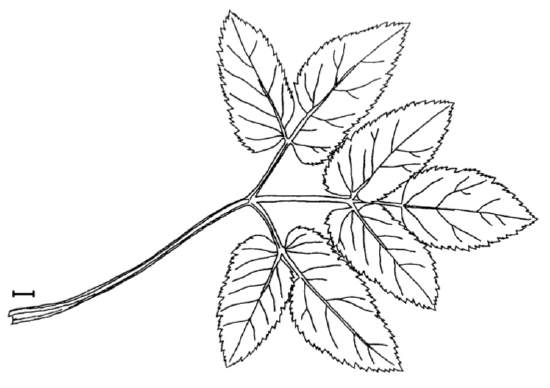 Figure \(\PageIndex{1}\) Leaf of Aegopodium podagraria., ground elder. Scale bar is approximately 10 mm.
First, check data, load it and check the object:
Code \(\PageIndex{12}\) (R):
(We also converted SUN variable into factor and supplied the proper labels.)
Let us check the data for the normality and for the most different character (Figure \(\PageIndex{2}\)):
Code \(\PageIndex{13}\) (R):
TERM.L (length of the terminal leaflet, it is the rightmost one on Figure \(\PageIndex{1}\)), is likely most different between sun and shade. Since this character is normal, we will run more precise parametric test:
Code \(\PageIndex{14}\) (R):
To report t-test result, one needs to provide degrees of freedom, statistic and p-value, e.g., like “in a Welch test, t statistic is 14.85 on 63.69 degrees of freedom, p-value is close to zero, thus we rejected the null hypothesis”.
Effect sizes are usually concerted with p-values but provide additional useful information about the magnitude of differences:
Code \(\PageIndex{15}\) (R):
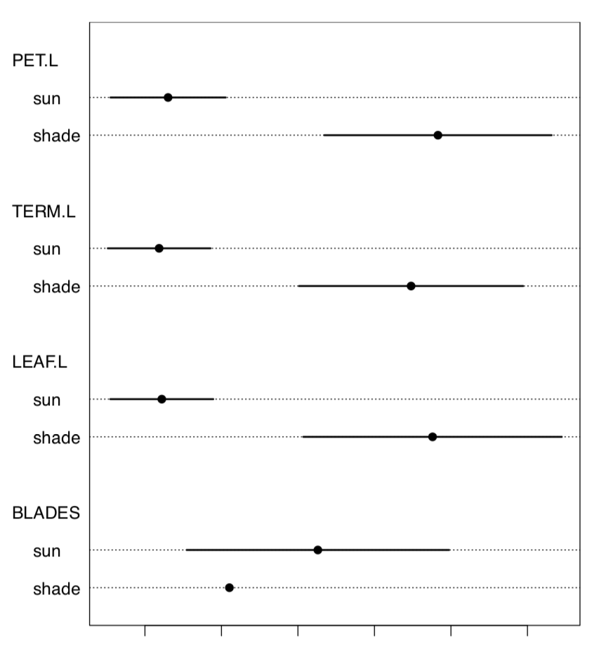 Figure \(\PageIndex{2}\) Medians with MADs in leaves data.
Both Cohen’s d and Lyubishchev’s K (coefficient of divergence) are large.
ANOVA
Answer to the height and color questions. Yes on both questions:
Code \(\PageIndex{16}\) (R):
There are significant differences between all three groups.
Answer to the question about differences between cow-wheats (Figure \(\PageIndex{3}\)) from seven locations.
Load the data and check its structure:
Code \(\PageIndex{17}\) (R):
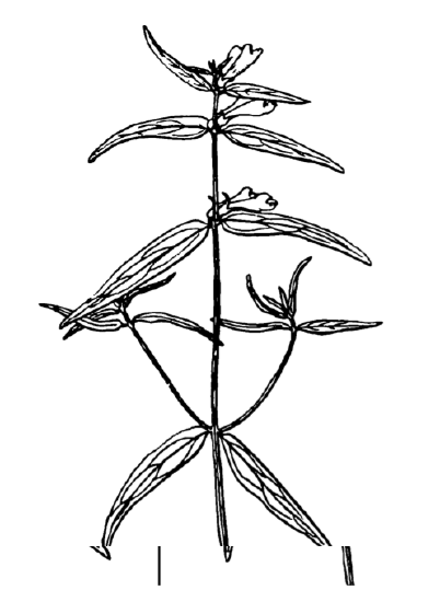 Figure \(\PageIndex{3}\) Top of the cow-wheat plant, Melampyrum sp. Size of fragment is approximately 10 cm.
Plot it first (Figure \(\PageIndex{4}\)):
Code \(\PageIndex{18}\) (R):
Check assumptions:
Code \(\PageIndex{19}\) (R):
Consequently, leaf length must be analyzed with non-parametric procedure, and plant height—with parametric which does not assume homogeneity of variance (one-way test):
Code \(\PageIndex{20}\) (R):
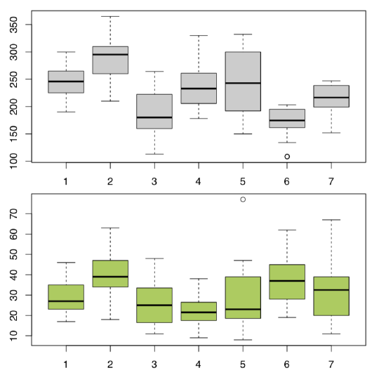 Figure \(\PageIndex{4}\) Cow-wheat stem heights (top) and leaf lengths (bottom) across seven different locations.
Now the leaf length:
Code \(\PageIndex{21}\) (R):
All in all, location pairs 2–4 and 4–6 are divergent statistically in both cases. This is visible also on boxplots (Figure \(\PageIndex{5}\)). There are more significant differences in plant heights, location #6, in particular, is quite outstanding.
Contingency tables
Answer to the seedlings question. Load data and check its structure:
Code \(\PageIndex{22}\) (R):
Now, what we need is to examine the table because both variables only look like numbers; in fact, they are categorical. Dotchart (Figure \(\PageIndex{5}\)) is a good way to explore 2-dimensional table:
Code \(\PageIndex{23}\) (R):
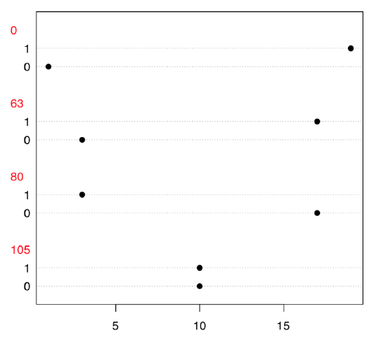 Figure \(\PageIndex{5}\) Dotchart to explore table made from seedlings data.
To explore possible associations visually, we employ vcd package:
Code \(\PageIndex{24}\) (R):
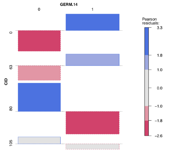 Figure \(\PageIndex{6}\) Advanced association plot of seedlings data.
Both table output and vcd association plot (Figure \(\PageIndex{6}\)) suggest some asymmetry (especially for CID80) which is a sign of possible association. Let us check it numerically, with the chi-squared test:
Code \(\PageIndex{25}\) (R):
Yes, there is an association between fungus (or their absence) and germination. How to know differences between particular samples? Here we need a post hoc test:
Code \(\PageIndex{26}\) (R):
(Exact Fisher test was used because some counts were really small.)
It is now clear that germination patterns form two fungal infections, CID80 and CID105, are significantly different from germination in the control (CID0). Also, significant association was found in the every comparison between three infections; this means that all three germination patterns are statistically different. Finally, one fungus, CID63 produces germination pattern which is not statistically different from the control.
Answer to the question about multiple comparisons of toxicity. Here we will go the slightly different way. Instead of using array, we will extract p-values right from the original data, and will avoid warnings with the exact test:
Code \(\PageIndex{27}\) (R):
(We cannot use pairwise.Table2.test() from the previous answer since our comparisons have different structure. But we used exact test to avoid warnings related with small numbers of counts.)
Now we can adjust p-values:
Code \(\PageIndex{28}\) (R):
Well, now we can say that Caesar salad and tomatoes are statistically supported as culprits. But why table tests always show us two factors? This could be due to the interaction: in simple words, it means that people who took the salad, frequently took tomatoes with it.
Answer to the scurvy-grass question. Check the data file, load and check result:
Code \(\PageIndex{29}\) (R):
(In addition, we converted LOC and IS.CREEPING to factors and provided new level labels.)
Next step is the visual analysis (Figure \(\PageIndex{7}\)):
Code \(\PageIndex{30}\) (R):
Some locations look different. To analyze, we need contingency table:
Code \(\PageIndex{31}\) (R):
Now the test and effect size:
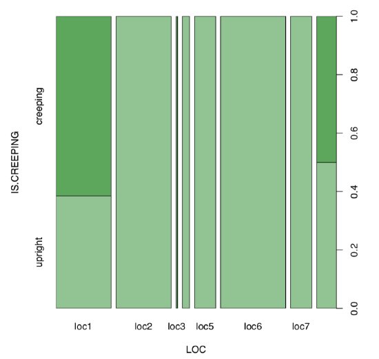 Figure \(\PageIndex{7}\) Spine plot: locality vs. life form of scurvy-grass.
Code \(\PageIndex{32}\) (R):
(Run pairwise.Table2.test(cc.lc) yourself to understand differences in details.)
Yes, there is a large, statistically significant association between locality and life form of scurvy-grass.
Answer to the question about equality of proportions of LOBES character in two birch localities. First, we need to select these two localities (1 and 2) and count proportions there. The shortest way is to use the table() function:
Code \(\PageIndex{33}\) (R):
Spine plot (Figure \(\PageIndex{8}\)) helps to make differences in the table even more apparent:
Code \(\PageIndex{34}\) (R):
(Please also note how to create two colors intermediate between black and dark green.)
The most natural choice is prop.test() which is applicable directly to the table() output:
Code \(\PageIndex{35}\) (R):
Instead of proportion test, we can use Fisher exact:
Code \(\PageIndex{36}\) (R):
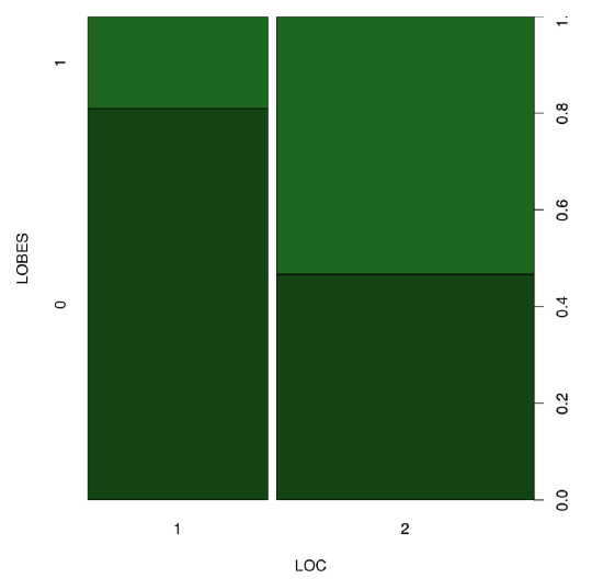 Figure \(\PageIndex{8}\) Spine plot of two birch characters.
... or chi-squared with simulation (note that one cell has only 4 cases), or with default Yates’ correction:
Code \(\PageIndex{37}\) (R):
All in all, yes, proportions of plants with different position of lobes are different between location 1 and 2.
And what about effect size of this association?
Code \(\PageIndex{38}\) (R):
Answer to the question about proportion equality in the whole betula dataset. First, make table:
Code \(\PageIndex{39}\) (R):
There is no apparent asymmetry. Since betula.lw is \(2\times2\) table, we can apply fourfold plot. It shows differences not only as different sizes of sectors, but also allows to check 95% confidence interval with marginal rings (Figure \(\PageIndex{9}\)):
Code \(\PageIndex{40}\) (R):
Also not suggestive... Finally, we need to test the association, if any. Noe that samples are related. This is because LOBES and WINGS were measured on the same plants. Therefore, instead of the chi-squared or proportion test we should run McNemar’s test:
Code \(\PageIndex{41}\) (R):
We conclude that proportions of two character states in each of characters are not statistically different.
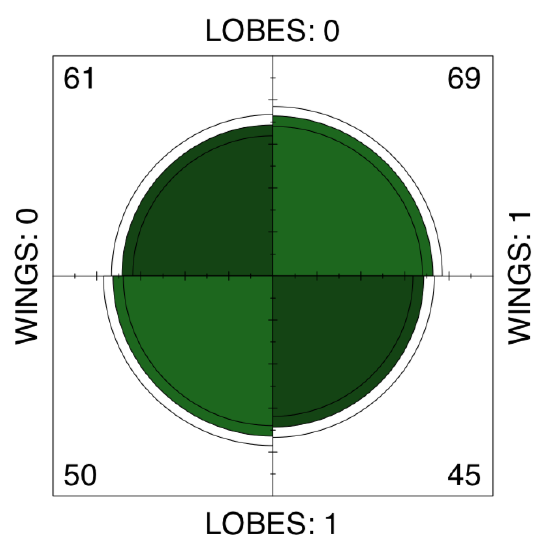 Figure \(\PageIndex{9}\) Fourfold plot of two birch characters.


