1.6.8.1: How to draw the multivariate data
- Page ID
- 32652
\( \newcommand{\vecs}[1]{\overset { \scriptstyle \rightharpoonup} {\mathbf{#1}} } \)
\( \newcommand{\vecd}[1]{\overset{-\!-\!\rightharpoonup}{\vphantom{a}\smash {#1}}} \)
\( \newcommand{\id}{\mathrm{id}}\) \( \newcommand{\Span}{\mathrm{span}}\)
( \newcommand{\kernel}{\mathrm{null}\,}\) \( \newcommand{\range}{\mathrm{range}\,}\)
\( \newcommand{\RealPart}{\mathrm{Re}}\) \( \newcommand{\ImaginaryPart}{\mathrm{Im}}\)
\( \newcommand{\Argument}{\mathrm{Arg}}\) \( \newcommand{\norm}[1]{\| #1 \|}\)
\( \newcommand{\inner}[2]{\langle #1, #2 \rangle}\)
\( \newcommand{\Span}{\mathrm{span}}\)
\( \newcommand{\id}{\mathrm{id}}\)
\( \newcommand{\Span}{\mathrm{span}}\)
\( \newcommand{\kernel}{\mathrm{null}\,}\)
\( \newcommand{\range}{\mathrm{range}\,}\)
\( \newcommand{\RealPart}{\mathrm{Re}}\)
\( \newcommand{\ImaginaryPart}{\mathrm{Im}}\)
\( \newcommand{\Argument}{\mathrm{Arg}}\)
\( \newcommand{\norm}[1]{\| #1 \|}\)
\( \newcommand{\inner}[2]{\langle #1, #2 \rangle}\)
\( \newcommand{\Span}{\mathrm{span}}\) \( \newcommand{\AA}{\unicode[.8,0]{x212B}}\)
\( \newcommand{\vectorA}[1]{\vec{#1}} % arrow\)
\( \newcommand{\vectorAt}[1]{\vec{\text{#1}}} % arrow\)
\( \newcommand{\vectorB}[1]{\overset { \scriptstyle \rightharpoonup} {\mathbf{#1}} } \)
\( \newcommand{\vectorC}[1]{\textbf{#1}} \)
\( \newcommand{\vectorD}[1]{\overrightarrow{#1}} \)
\( \newcommand{\vectorDt}[1]{\overrightarrow{\text{#1}}} \)
\( \newcommand{\vectE}[1]{\overset{-\!-\!\rightharpoonup}{\vphantom{a}\smash{\mathbf {#1}}}} \)
\( \newcommand{\vecs}[1]{\overset { \scriptstyle \rightharpoonup} {\mathbf{#1}} } \)
\( \newcommand{\vecd}[1]{\overset{-\!-\!\rightharpoonup}{\vphantom{a}\smash {#1}}} \)
\(\newcommand{\avec}{\mathbf a}\) \(\newcommand{\bvec}{\mathbf b}\) \(\newcommand{\cvec}{\mathbf c}\) \(\newcommand{\dvec}{\mathbf d}\) \(\newcommand{\dtil}{\widetilde{\mathbf d}}\) \(\newcommand{\evec}{\mathbf e}\) \(\newcommand{\fvec}{\mathbf f}\) \(\newcommand{\nvec}{\mathbf n}\) \(\newcommand{\pvec}{\mathbf p}\) \(\newcommand{\qvec}{\mathbf q}\) \(\newcommand{\svec}{\mathbf s}\) \(\newcommand{\tvec}{\mathbf t}\) \(\newcommand{\uvec}{\mathbf u}\) \(\newcommand{\vvec}{\mathbf v}\) \(\newcommand{\wvec}{\mathbf w}\) \(\newcommand{\xvec}{\mathbf x}\) \(\newcommand{\yvec}{\mathbf y}\) \(\newcommand{\zvec}{\mathbf z}\) \(\newcommand{\rvec}{\mathbf r}\) \(\newcommand{\mvec}{\mathbf m}\) \(\newcommand{\zerovec}{\mathbf 0}\) \(\newcommand{\onevec}{\mathbf 1}\) \(\newcommand{\real}{\mathbb R}\) \(\newcommand{\twovec}[2]{\left[\begin{array}{r}#1 \\ #2 \end{array}\right]}\) \(\newcommand{\ctwovec}[2]{\left[\begin{array}{c}#1 \\ #2 \end{array}\right]}\) \(\newcommand{\threevec}[3]{\left[\begin{array}{r}#1 \\ #2 \\ #3 \end{array}\right]}\) \(\newcommand{\cthreevec}[3]{\left[\begin{array}{c}#1 \\ #2 \\ #3 \end{array}\right]}\) \(\newcommand{\fourvec}[4]{\left[\begin{array}{r}#1 \\ #2 \\ #3 \\ #4 \end{array}\right]}\) \(\newcommand{\cfourvec}[4]{\left[\begin{array}{c}#1 \\ #2 \\ #3 \\ #4 \end{array}\right]}\) \(\newcommand{\fivevec}[5]{\left[\begin{array}{r}#1 \\ #2 \\ #3 \\ #4 \\ #5 \\ \end{array}\right]}\) \(\newcommand{\cfivevec}[5]{\left[\begin{array}{c}#1 \\ #2 \\ #3 \\ #4 \\ #5 \\ \end{array}\right]}\) \(\newcommand{\mattwo}[4]{\left[\begin{array}{rr}#1 \amp #2 \\ #3 \amp #4 \\ \end{array}\right]}\) \(\newcommand{\laspan}[1]{\text{Span}\{#1\}}\) \(\newcommand{\bcal}{\cal B}\) \(\newcommand{\ccal}{\cal C}\) \(\newcommand{\scal}{\cal S}\) \(\newcommand{\wcal}{\cal W}\) \(\newcommand{\ecal}{\cal E}\) \(\newcommand{\coords}[2]{\left\{#1\right\}_{#2}}\) \(\newcommand{\gray}[1]{\color{gray}{#1}}\) \(\newcommand{\lgray}[1]{\color{lightgray}{#1}}\) \(\newcommand{\rank}{\operatorname{rank}}\) \(\newcommand{\row}{\text{Row}}\) \(\newcommand{\col}{\text{Col}}\) \(\renewcommand{\row}{\text{Row}}\) \(\newcommand{\nul}{\text{Nul}}\) \(\newcommand{\var}{\text{Var}}\) \(\newcommand{\corr}{\text{corr}}\) \(\newcommand{\len}[1]{\left|#1\right|}\) \(\newcommand{\bbar}{\overline{\bvec}}\) \(\newcommand{\bhat}{\widehat{\bvec}}\) \(\newcommand{\bperp}{\bvec^\perp}\) \(\newcommand{\xhat}{\widehat{\xvec}}\) \(\newcommand{\vhat}{\widehat{\vvec}}\) \(\newcommand{\uhat}{\widehat{\uvec}}\) \(\newcommand{\what}{\widehat{\wvec}}\) \(\newcommand{\Sighat}{\widehat{\Sigma}}\) \(\newcommand{\lt}{<}\) \(\newcommand{\gt}{>}\) \(\newcommand{\amp}{&}\) \(\definecolor{fillinmathshade}{gray}{0.9}\)The most simple operation with multidimensional data is to draw it.
Pictographs
Pictograph is a plot where each element represents one of objects, and every feature of the element corresponds with one character of the primary object. If the every row of data is unique, pictographs might be useful. Here is the star plot (Figure \(\PageIndex{1}\)) example:
Code \(\PageIndex{1}\) (R):
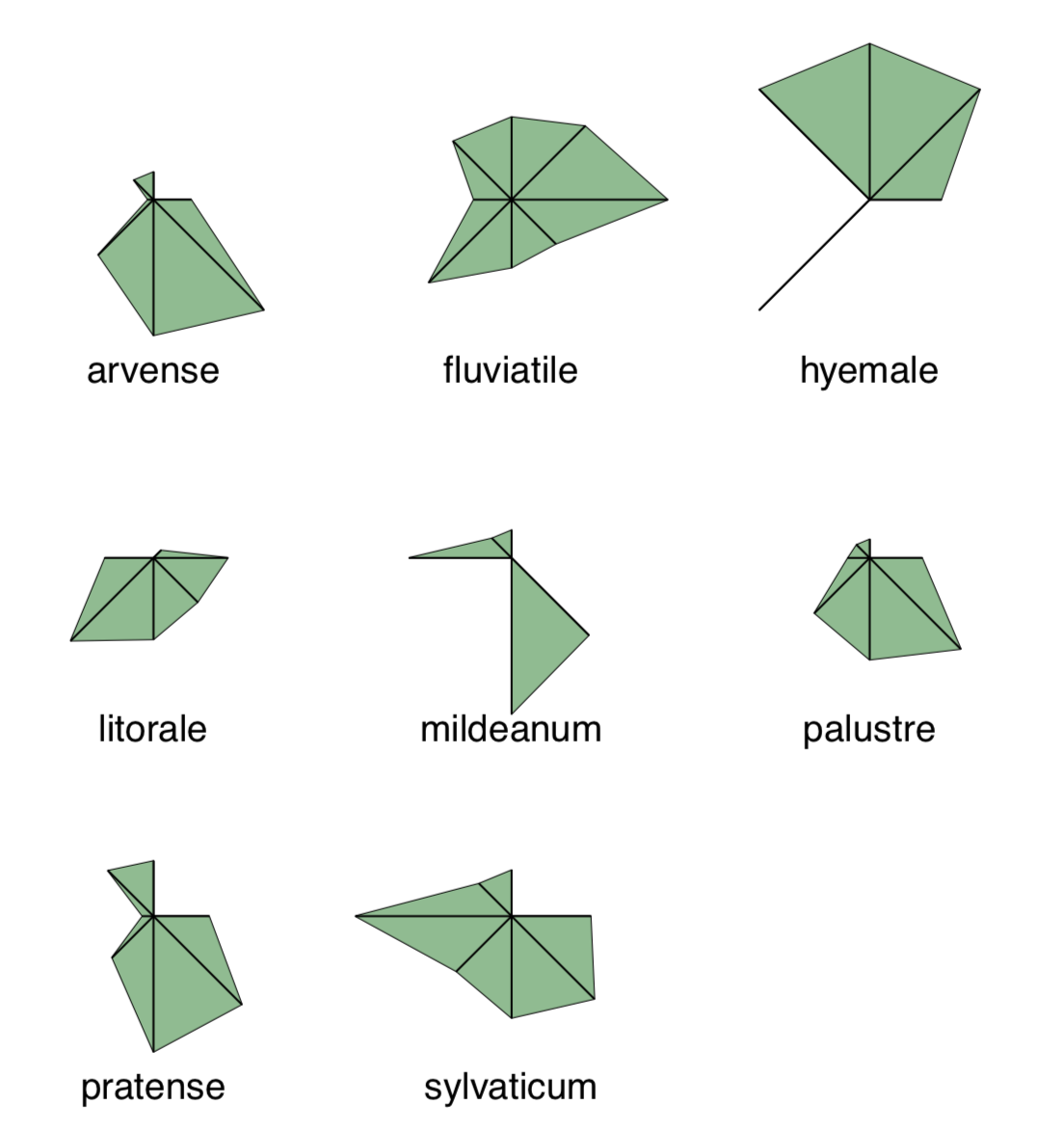 Figure \(\PageIndex{1}\) Stars show different horsetail species.
(We made every element to represent the species of horsetails, and length of the particular ray corresponds with some morphological characters. It is easy to see, as an example, similarities between Equisetum \(\times\)litorale and E. fluviatile.)
Slightly more exotic pictograph is Chernoff’s faces where features of elements are shown as human face characters (Figure \(\PageIndex{1}\)):
Code \(\PageIndex{2}\) (R):
(Original Chernoff’s faces have been implemented in the faces2() function, there is also another variant in symbols() package.)
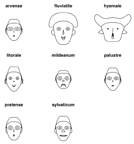 Figure \(\PageIndex{2}\) Chernoff’s faces show different horsetail species.
Related to pictographs are ways to overview the whole numeric dataset, matrix or data frame. First, command image() allows for plots like on Figure \(\PageIndex{3}\):
Code \(\PageIndex{3}\) (R):
(This is a “portrait” or iris matrix, not extremely informative but useful in many ways. For example, it is well visible that highest, most red, values of Pt.L (abbreviated from Petal.Length) correspond with lowest values of Sp.W (Sepal.Width). It is possible even to spot 3-species structure of this data.)
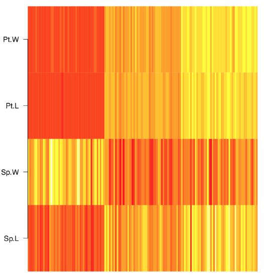 Figure \(\PageIndex{3}\) Results of plotting iris data with the image() command. Redder colors correspond with higher values of scaled characters.
More advanced is the parallel coordinates plot (Figure \(\PageIndex{4}\)):
Code \(\PageIndex{4}\) (R):
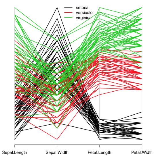 Figure \(\PageIndex{4}\) Parallel coordinates plot.
This is somewhat like the multidimensional stripchart. Every character is represented with one axis which has its values from all plants. Then, for every plant, these values were connected with lines. There are many interesting things which could be spotted from this plot. For example, it is clear that petal characters are more distinguishing than sepal. It is also visible that Iris setosa is more distinct from two other species, and so on.
Grouped plots
Even boxplots and dotcharts could represent multiple characters of multiple groups, but you will need to scale them first and then manually control positions of plotted elements, or use Boxplots() and Linechart() described in the previous chapter:
Code \(\PageIndex{5}\) (R):
(Please try these plots yourself.)
Function matplot() allows to place multiple scatterplots in one frame, symbols() allows to place multiple smaller plots in desired locations, and function pairs() allows to show multiple scatterplots as a matrix (Figure \(\PageIndex{5}\)).
Code \(\PageIndex{6}\) (R):
(This matrix plot shows dependencies between each possible pair of five variables simultaneously.)
Matrix plot is just one of the big variety of R trellis plots. Many of them are in the lattice package (Figure \(\PageIndex{6}\)):
Code \(\PageIndex{7}\) (R):
(Note how to use make.groups() and do.call() to stack all columns into the long variable (it is also possible to use stack(), see above). When LOC was added to temporary dataset, it was recycled five times—exactly what we need.)
Library lattice offers multiple trellis variants of common R plots. For example, one could make the trellis dotchart which will show differences between horsetail species (Figure \(\PageIndex{7}\))
Code \(\PageIndex{8}\) (R):
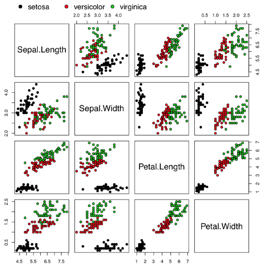 Figure \(\PageIndex{5}\) Matrix plot.
(Here we stacked all numerical columns into one with stack().)
Few trellis plots are available in the core R. This is our election data from previous chapter (Figure \(\PageIndex{8}\)):
Code \(\PageIndex{9}\) (R):
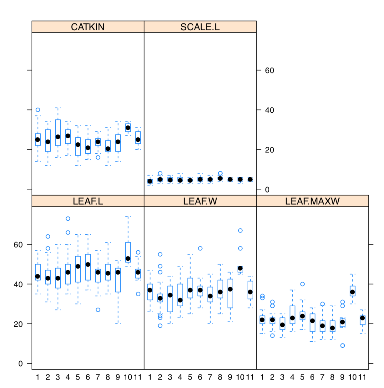 Figure \(\PageIndex{6}\) The example of trellis plot: for each measurement character, boxplots represent differences between locations.
3D plots
If there just three numerical variables, we can try to plot all of them with 3-axis plots. Frequently seen in geology, metallurgy and some other fields are ternary plots. They implemented, for example, in the vcd package. They use triangle coordinate system which allows to reflect simultaneously three measurement variables and some more categorical characters (via colors, point types etc.):
Code \(\PageIndex{10}\) (R):
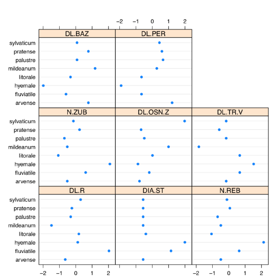 Figure \(\PageIndex{7}\) Trellis dotchart of the horsetail species (character values are scaled). These plots are typically read from the bottom.
The “brick” 3D plot could be done, for example, with the package scatterplot3d (Figure \(\PageIndex{10}\)):
Code \(\PageIndex{11}\) (R):
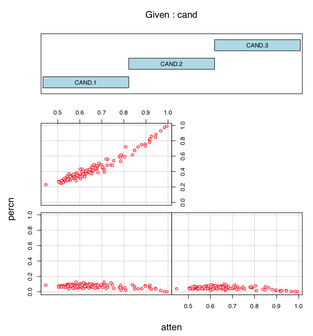 Figure \(\PageIndex{8}\) Voting data from previous chapter represented with coplot() function.
(Here some additional efforts were used to make y-axis label slanted.)
These 3D scatterplots look attractive, but what if some points were hidden from the view? How to rotate and find the best projection? Library RGL will help to create the dynamic 3D plot:
Code \(\PageIndex{12}\) (R):
Please run these commands yourself. The size of window and projection in RGL plots are controlled with mouse. That will help to understand better the position of every point. In case of iris data, it is visible clearly that one of the species (Iris setosa) is more distinct than two others, and the most “splitting” character is the length of petals (Petal.Length). There are four characters on the plot, because color was used to distinguish species. To save current RGL plot, you will need to run rgl.snapshot() or rgl.postscript() function. Please also note that RGL package depends on the external OpenGL library and therefore on some systems, additional installations might be required.
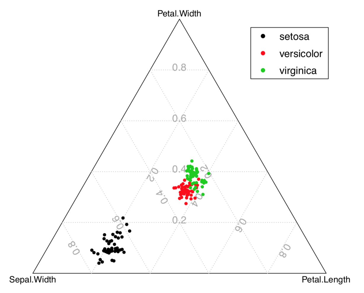 Figure \(\PageIndex{9}\) Ternary plot for iris data.
Another 3D possibility is cloud() from lattice package. It is a static plot with the relatively heavy code but important is that user can use different rotations (Figure 7.2.1):
Code \(\PageIndex{13}\) (R):
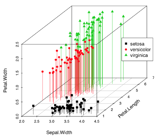 Figure \(\PageIndex{10}\) Static 3D scatterplot of iris data.


