1.6.8.3: Machine learning
- Page ID
- 32654
\( \newcommand{\vecs}[1]{\overset { \scriptstyle \rightharpoonup} {\mathbf{#1}} } \)
\( \newcommand{\vecd}[1]{\overset{-\!-\!\rightharpoonup}{\vphantom{a}\smash {#1}}} \)
\( \newcommand{\id}{\mathrm{id}}\) \( \newcommand{\Span}{\mathrm{span}}\)
( \newcommand{\kernel}{\mathrm{null}\,}\) \( \newcommand{\range}{\mathrm{range}\,}\)
\( \newcommand{\RealPart}{\mathrm{Re}}\) \( \newcommand{\ImaginaryPart}{\mathrm{Im}}\)
\( \newcommand{\Argument}{\mathrm{Arg}}\) \( \newcommand{\norm}[1]{\| #1 \|}\)
\( \newcommand{\inner}[2]{\langle #1, #2 \rangle}\)
\( \newcommand{\Span}{\mathrm{span}}\)
\( \newcommand{\id}{\mathrm{id}}\)
\( \newcommand{\Span}{\mathrm{span}}\)
\( \newcommand{\kernel}{\mathrm{null}\,}\)
\( \newcommand{\range}{\mathrm{range}\,}\)
\( \newcommand{\RealPart}{\mathrm{Re}}\)
\( \newcommand{\ImaginaryPart}{\mathrm{Im}}\)
\( \newcommand{\Argument}{\mathrm{Arg}}\)
\( \newcommand{\norm}[1]{\| #1 \|}\)
\( \newcommand{\inner}[2]{\langle #1, #2 \rangle}\)
\( \newcommand{\Span}{\mathrm{span}}\) \( \newcommand{\AA}{\unicode[.8,0]{x212B}}\)
\( \newcommand{\vectorA}[1]{\vec{#1}} % arrow\)
\( \newcommand{\vectorAt}[1]{\vec{\text{#1}}} % arrow\)
\( \newcommand{\vectorB}[1]{\overset { \scriptstyle \rightharpoonup} {\mathbf{#1}} } \)
\( \newcommand{\vectorC}[1]{\textbf{#1}} \)
\( \newcommand{\vectorD}[1]{\overrightarrow{#1}} \)
\( \newcommand{\vectorDt}[1]{\overrightarrow{\text{#1}}} \)
\( \newcommand{\vectE}[1]{\overset{-\!-\!\rightharpoonup}{\vphantom{a}\smash{\mathbf {#1}}}} \)
\( \newcommand{\vecs}[1]{\overset { \scriptstyle \rightharpoonup} {\mathbf{#1}} } \)
\( \newcommand{\vecd}[1]{\overset{-\!-\!\rightharpoonup}{\vphantom{a}\smash {#1}}} \)
\(\newcommand{\avec}{\mathbf a}\) \(\newcommand{\bvec}{\mathbf b}\) \(\newcommand{\cvec}{\mathbf c}\) \(\newcommand{\dvec}{\mathbf d}\) \(\newcommand{\dtil}{\widetilde{\mathbf d}}\) \(\newcommand{\evec}{\mathbf e}\) \(\newcommand{\fvec}{\mathbf f}\) \(\newcommand{\nvec}{\mathbf n}\) \(\newcommand{\pvec}{\mathbf p}\) \(\newcommand{\qvec}{\mathbf q}\) \(\newcommand{\svec}{\mathbf s}\) \(\newcommand{\tvec}{\mathbf t}\) \(\newcommand{\uvec}{\mathbf u}\) \(\newcommand{\vvec}{\mathbf v}\) \(\newcommand{\wvec}{\mathbf w}\) \(\newcommand{\xvec}{\mathbf x}\) \(\newcommand{\yvec}{\mathbf y}\) \(\newcommand{\zvec}{\mathbf z}\) \(\newcommand{\rvec}{\mathbf r}\) \(\newcommand{\mvec}{\mathbf m}\) \(\newcommand{\zerovec}{\mathbf 0}\) \(\newcommand{\onevec}{\mathbf 1}\) \(\newcommand{\real}{\mathbb R}\) \(\newcommand{\twovec}[2]{\left[\begin{array}{r}#1 \\ #2 \end{array}\right]}\) \(\newcommand{\ctwovec}[2]{\left[\begin{array}{c}#1 \\ #2 \end{array}\right]}\) \(\newcommand{\threevec}[3]{\left[\begin{array}{r}#1 \\ #2 \\ #3 \end{array}\right]}\) \(\newcommand{\cthreevec}[3]{\left[\begin{array}{c}#1 \\ #2 \\ #3 \end{array}\right]}\) \(\newcommand{\fourvec}[4]{\left[\begin{array}{r}#1 \\ #2 \\ #3 \\ #4 \end{array}\right]}\) \(\newcommand{\cfourvec}[4]{\left[\begin{array}{c}#1 \\ #2 \\ #3 \\ #4 \end{array}\right]}\) \(\newcommand{\fivevec}[5]{\left[\begin{array}{r}#1 \\ #2 \\ #3 \\ #4 \\ #5 \\ \end{array}\right]}\) \(\newcommand{\cfivevec}[5]{\left[\begin{array}{c}#1 \\ #2 \\ #3 \\ #4 \\ #5 \\ \end{array}\right]}\) \(\newcommand{\mattwo}[4]{\left[\begin{array}{rr}#1 \amp #2 \\ #3 \amp #4 \\ \end{array}\right]}\) \(\newcommand{\laspan}[1]{\text{Span}\{#1\}}\) \(\newcommand{\bcal}{\cal B}\) \(\newcommand{\ccal}{\cal C}\) \(\newcommand{\scal}{\cal S}\) \(\newcommand{\wcal}{\cal W}\) \(\newcommand{\ecal}{\cal E}\) \(\newcommand{\coords}[2]{\left\{#1\right\}_{#2}}\) \(\newcommand{\gray}[1]{\color{gray}{#1}}\) \(\newcommand{\lgray}[1]{\color{lightgray}{#1}}\) \(\newcommand{\rank}{\operatorname{rank}}\) \(\newcommand{\row}{\text{Row}}\) \(\newcommand{\col}{\text{Col}}\) \(\renewcommand{\row}{\text{Row}}\) \(\newcommand{\nul}{\text{Nul}}\) \(\newcommand{\var}{\text{Var}}\) \(\newcommand{\corr}{\text{corr}}\) \(\newcommand{\len}[1]{\left|#1\right|}\) \(\newcommand{\bbar}{\overline{\bvec}}\) \(\newcommand{\bhat}{\widehat{\bvec}}\) \(\newcommand{\bperp}{\bvec^\perp}\) \(\newcommand{\xhat}{\widehat{\xvec}}\) \(\newcommand{\vhat}{\widehat{\vvec}}\) \(\newcommand{\uhat}{\widehat{\uvec}}\) \(\newcommand{\what}{\widehat{\wvec}}\) \(\newcommand{\Sighat}{\widehat{\Sigma}}\) \(\newcommand{\lt}{<}\) \(\newcommand{\gt}{>}\) \(\newcommand{\amp}{&}\) \(\definecolor{fillinmathshade}{gray}{0.9}\)Methods explained in this section are not only visualizations. Together, they frequently called “classification with learning”, “supervised classification”, “machine learning”, or just “classification”. All of them are based on the idea of learning:
... He scrambled through and rose to his feet. ... He saw nothing but colours—colours that refused to form themselves into things. Moreover, he knew nothing yet well enough to see it: you cannot see things till you know roughly what they are\(^{[1]}\). His first impression was of a bright, pale world—a watercolour world out
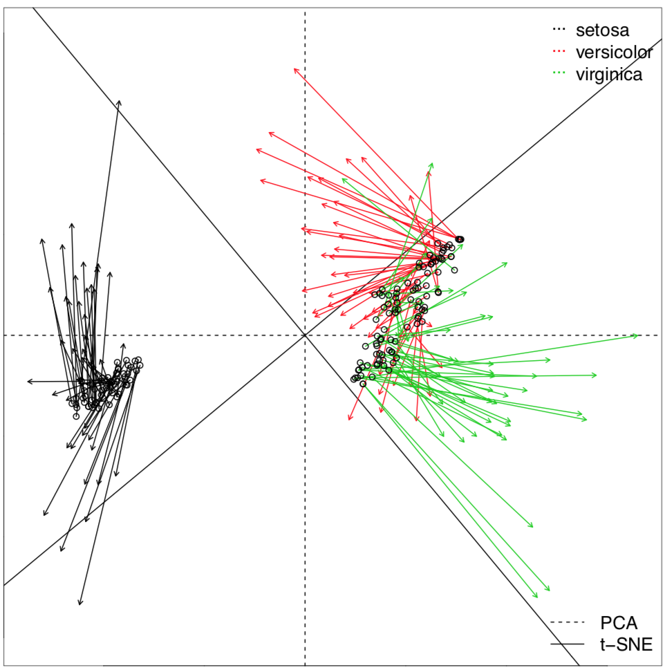 Figure \(\PageIndex{1}\) Procrustes plot which show t-SNE ordination against the target PCA ordination.
of a child’s paint-box; a moment later he recognized the flat belt of light blue as a sheet of water, or of something like water, which came nearly to his feet. They were on the shore of a lake or river...
C.S.Lewis. Out of the Silent Planet.
First, small part of data where identity is already known (training dataset) used to develop (fit) the model of classification (Figure \(\PageIndex{2}\)). On the next step, this model is used to classify objects with unknown identity (testing dataset). In most of these methods, it is possible to estimate the quality of the classification and also assess the significance of the every character.
Let us create training and testing datasets from iris data:
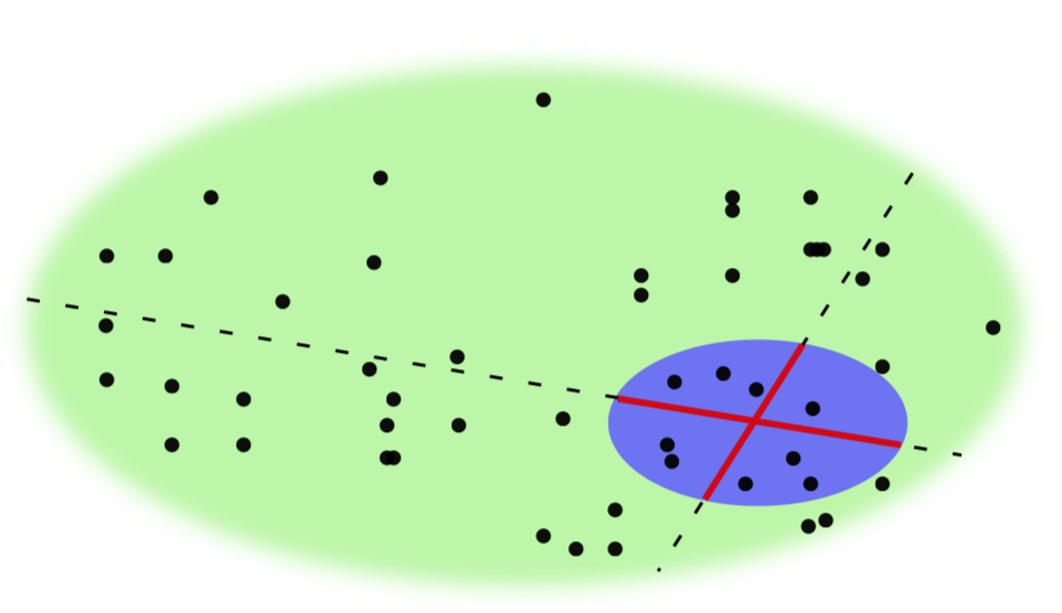 Figure \(\PageIndex{2}\) Graphic representation of the statistical machine learning. Blue is a training dataset, red lines is classification model, green is a testing dataset, dashed lines show prediction (estimation) process.
Code \(\PageIndex{1}\) (R):
(iris.unknown is of course the fake unknown so to use it properly, we must specify iris.unknown[, -5]. On the other hand, species information will help to create misclassification table (confusion matrix, see below).)
Learning with regression
Linear discriminant analysis
One of the simplest methods of classification is the linear discriminant analysis (LDA). The basic idea is to create the set of linear functions which “decide” how to classify the particular object.
Code \(\PageIndex{2}\) (R):
Training resulted in the hypothesis which allowed almost all plants (with an exception of seven Iris virginica) to be placed into the proper group. Please note that LDA does not require scaling of variables.
It is possible to check LDA results with inferential methods. Multidimensional analysis of variation (MANOVA) allows to understand the relation between data and model (classification from LDA):
Code \(\PageIndex{3}\) (R):
Important here are both p-value based on Fisher statistics, and also the value of Wilks’ statistics which is the likelihood ratio (in our case, the probability that groups are not different).
It is possible to check the relative importance of every character in LDA with ANOVA-like techniques:
Code \(\PageIndex{4}\) (R):
(This idea is applicable to other classification methods too.)
... and also visualize LDA results (Figure \(\PageIndex{3}\)):
Code \(\PageIndex{5}\) (R):
(Please note 95% confidence ellipses with centers.)
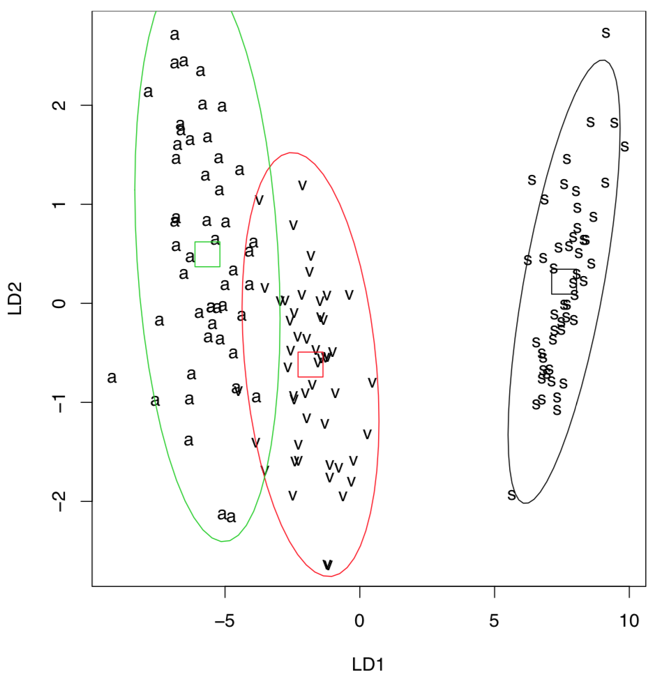 Figure \(\PageIndex{3}\) Graphical representation of the linear discriminant analysis results. 95% confidence ellipses and their centers added with Ellipses() function.
To place all points on the plot, we simply used all data as training. Note the good discrimination (higher than in PCA, MDS or clustering), even between close Iris versicolor and I. virginica. This is because LDA frequently overestimates the differences between groups. This feature, and also the parametricity and linearity of LDA made it less used over the last years.
With LDA, it is easy to illustrate one more important concept of machine learning: quality of training. Consider the following example:
Code \(\PageIndex{6}\) (R):
Misclassification error here almost two times bigger! Why?
Code \(\PageIndex{7}\) (R):
Well, using sample() (and particular set.seed() value) resulted in biased training sample, this is why our second model was trained so poorly. Our first way to sample (every 5th iris) was better, and if there is a need to use sample(), consider to sample each species separately.
Now, return to the default random number generator settings:
Code \(\PageIndex{8}\) (R):
Please note that it is widely known that while LDA was developed on biological material, this kind of data rarely meets two key assumptions of this method: (1) multivariate normality and (2) multivariate homoscedasticity. Amazingly, even Fisher’s Iris data with which LDA was invented, does not meet these assumptions! Therefore, we do not recommend to use LDA and keep it here mostly for teaching purposes.
Recursive partitioning
To replace linear discriminant analysis, multiple methods with similar background ideas were invented. Recursive partitioning, or decision trees (regression trees, classification trees), allow, among other, to make and visualize the sort of discrimination key where every step results in splitting objects in two groups (Figure \(\PageIndex{4}\)):
Code \(\PageIndex{9}\) (R):
We loaded first the tree package containing tree() function (rpart is another package which makes classification trees). Then we again used the whole dataset as training data. The plot shows that all plants with petal length less than 2.45 cm belong to Iris setosa, and from the rest those plants which have petal width less than 1.75 cm and petal length more than 4.95 cm, are I. versicolor; all other irises belong to I. virginica.
In fact, these trees are result of something similar to “hierarchical discriminant analysis”, and it is possible to use them for the supervised classification:
Code \(\PageIndex{10}\) (R):
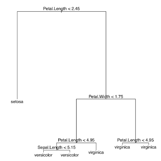 Figure \(\PageIndex{4}\) Classification tree for the iris data from tree package.
Try to find out which characters distinguish species of horsetails described in eq.txt data file. File eq_c.txt contains the description of characters.
Package party offers sophisticated recursive partitioning methods together with advanced tree plots (Figure \(\PageIndex{5}\)):
Code \(\PageIndex{11}\) (R):
(For species names, we used one-letter abbreviations.)
Ensemble learnig
Random Forest
The other method, internally similar to regression trees, rapidly gains popularity. This is the Random Forest. Its name came from the ability to use numerous decision trees and build the complex classification model. Random Forest belongs to bagging ensemble methods; it uses bootstrap (see in Appendix) to multiply the number of trees in the model (hence “forest”). Below is an example of Random Forest classifier made from the iris data:
Code \(\PageIndex{12}\) (R):
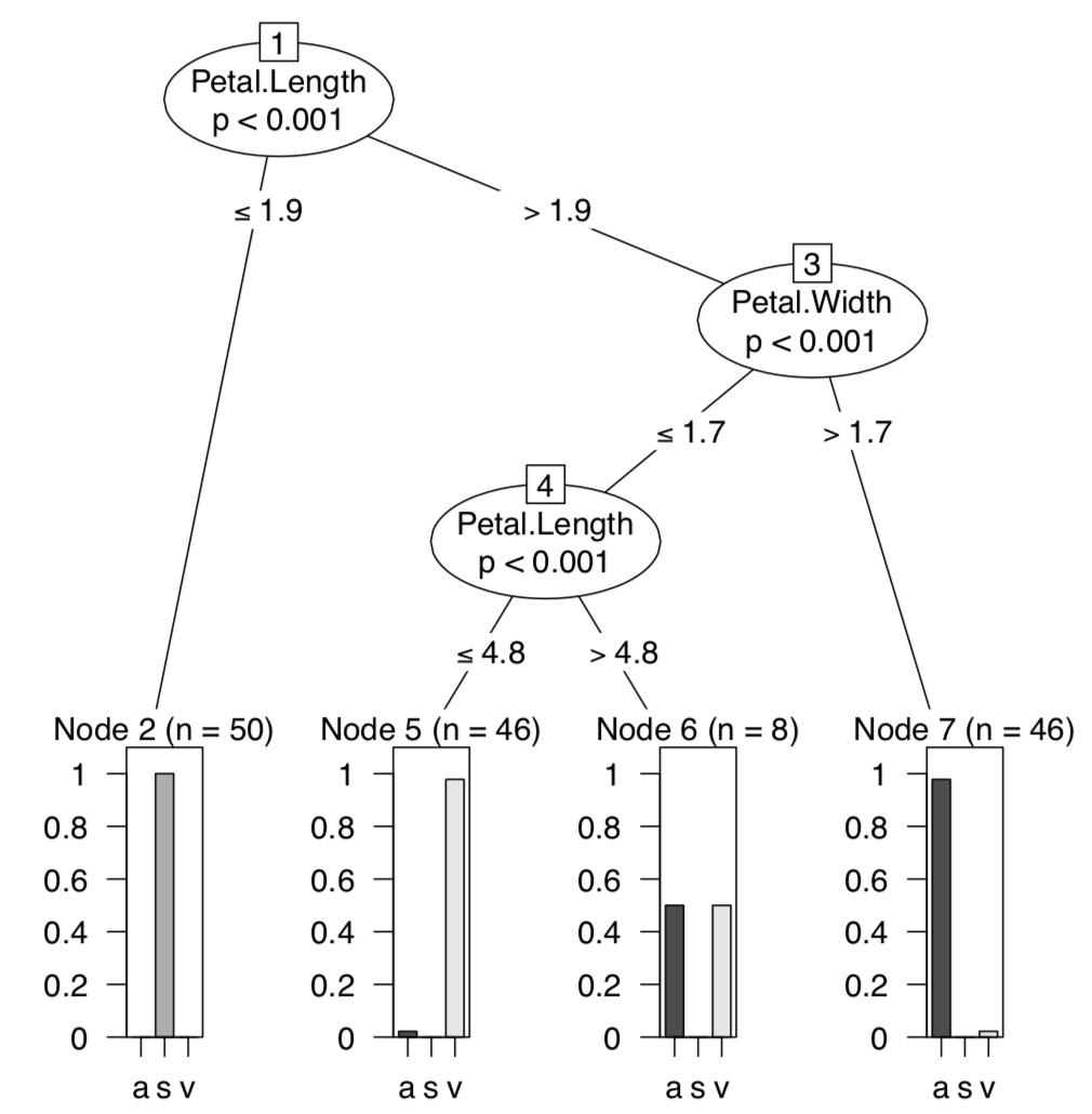 Figure \(\PageIndex{5}\) Classification tree for the iris data from party package.
Here results are similar to LDA but Random Forest allows for more. For example, it can clarify the importance of each character (with function importance()), and reveal classification distances (proximities) between all objects of training subset (these distances could be in turn used for clustering). Random Forest could also visualize the multidimensional dataset (Figure \(\PageIndex{6}\)):
Code \(\PageIndex{13}\) (R):
(We applied several tricks to show convex hulls and their centroids.)
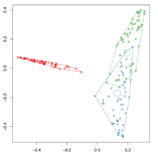 Figure \(\PageIndex{6}\) Visualization of iris data with the help of “Random Forest”. Hulls and their centroids added with Hulls() function.
Package ranger implements even faster variant of Random Forest algorithm, it also can employ parallel calculations.
Gradient boosting
There are many weak classification methods which typically make high misclassification errors. However, many of them are also ultra-fast. So, is it possible to combine many weak learners to make the strong one? Yes! This is what boosting methods do. Gradient boosting employs multi-step optimization and is now among most frequently using learning techniques. In R, there are several gradient boosting packages, for example, xgboost and gbm:
Code \(\PageIndex{14}\) (R):
(Plot is purely technical; in the above form, it will show the marginal effect (effect on membership) of the 1st variable. Please make it yourself. “Membership trick” selects the “best species” from three alternatives as gbm() reports classification result in fuzzy form.)
Learning with proximity
k-Nearest Neighbors algorithm (or kNN) is the “lazy classifier” because it does not work until unknown data is supplied:
Code \(\PageIndex{15}\) (R):
kNN is based on distance calculation and “voting”. It calculates distances from every unknown object to the every object of the training set. Next, it considers several (5 in the case above) nearest neighbors with known identity and finds which id is prevalent. This prevalent id assigned to the unknown member. Function knn() uses Euclidean distances but in principle, any distance would work for kNN.
To illustrate idea of nearest neighbors, we use Voronoi decomposition, the technique which is close to both kNN and distance calculation:
Code \(\PageIndex{16}\) (R):
The plot (Figure \(\PageIndex{7}\)) contains multiple cells which represent neighborhoods of training sample (big dots). This is not exactly what kNN does, but idea is just the same. In fact, Voronoi plot is a good tool to visualize any distance-based approach.
Depth classification based on how close an arbitrary point of the space is located to an implicitly defined center of a multidimensional data cloud:
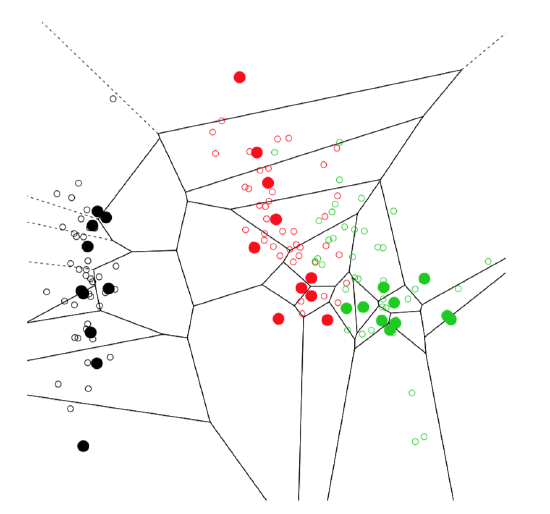 Figure \(\PageIndex{7}\) Visualization of training data points neighborhoods with Voronoi decomposition.
Code \(\PageIndex{17}\) (R):
Learning with rules
Naïve Bayes classifier is one of the simplest machine learning algorithms which tries to classify objects based on the probabilities of previously seen attributes. Quite unexpectedly, it is typically a good classifier:
Code \(\PageIndex{18}\) (R):
Note that Naïve Bayes classifier could use not only numerical like above, but also nominal predictors (which is similar to correspondence analysis.)
Apriori method is similar to regression trees but instead of classifying objects, it researches association rules between classes of objects. This method could be used not only to find these rules but also to make classification. Note that measurement iris data is less suitable for association rules then nominal data, and it needs discretization first:
Code \(\PageIndex{19}\) (R):
(Rules are self-explanatory. What do you think, does this method performs better for the nominal data? Please find it out.)
Learning from the black box
Famous SVM, Support Vector Machines is a kernel technique which calculates parameters of the hyper-planes dividing multiple groups in the multidimensional space of characters:
Code \(\PageIndex{20}\) (R):
Classification, or prediction grid often helps to illustrate the SVM method. Data points are arranged with PCA to reduce dimensionality, and then classifier predicts the identity for the every point in the artificially made grid (Figure \(\PageIndex{8}\)). This is possible to perform manually but Gradd() function simplifies plotting:
Code \(\PageIndex{21}\) (R):
And finally, neural networks! This name is used for the statistical technique based on some features of neural cells, neurons. First, we need to prepare data and convert categorical variable Species into three logical dummy variables:
Code \(\PageIndex{22}\) (R):
Now, we call neuralnet package and proceed to the main calculation. The package “wants” to supply all terms in the model explicitly:
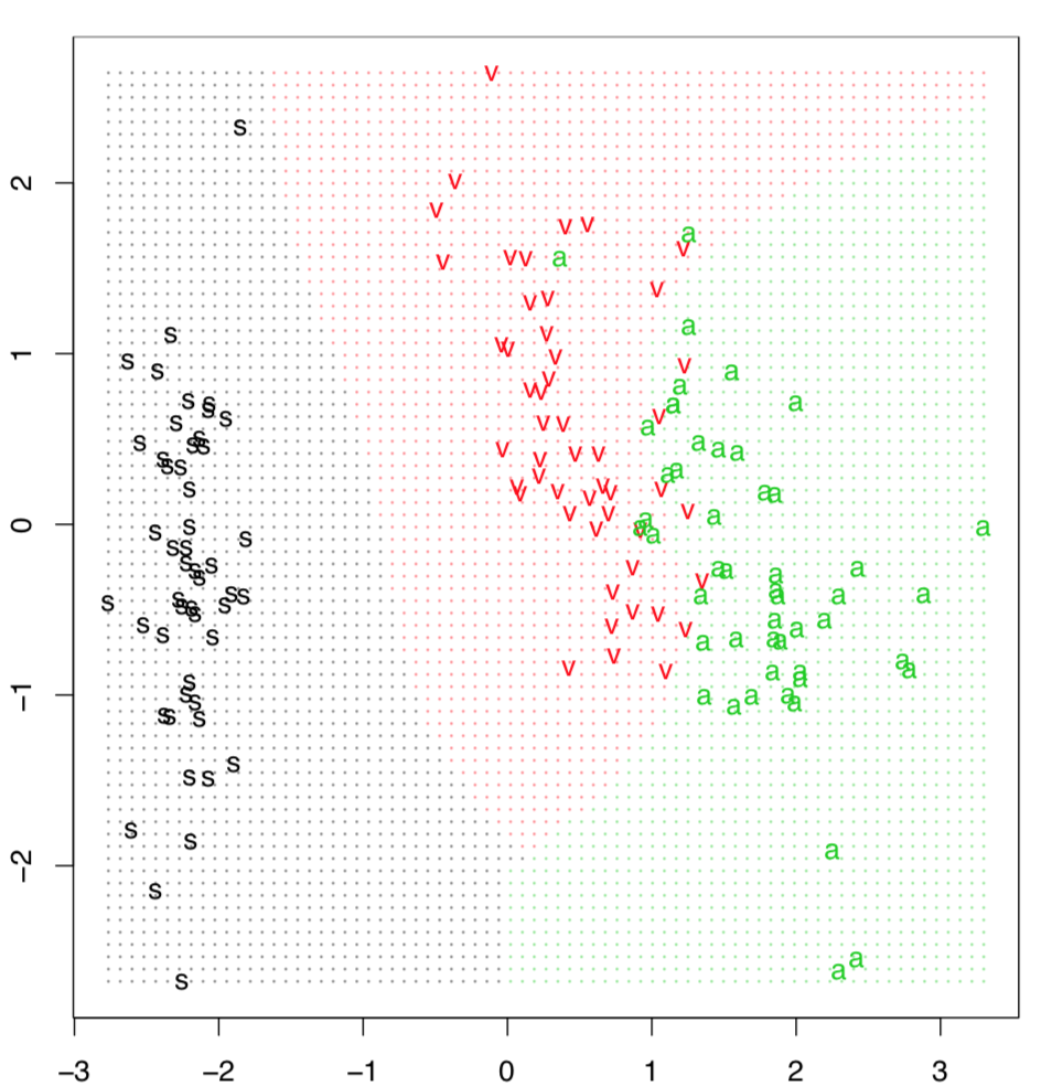 Figure \(\PageIndex{8}\) Classification grid which illustrates the SVM algorithm. Data points are arranged with PCA.
Code \(\PageIndex{23}\) (R):
(Note use of set.seed(), this is to make your results similar to presented here.)
Now predict (with compute() function) and check misclassification:
Code \(\PageIndex{24}\) (R):
Results of neural network prediction are fuzzy, similar to the results of fuzzy clustering or regression trees, this is why which.max() was applied for every row. As you see, this is one of the lowest misclassification errors.
It is possible to plot the actual network:
Code \(\PageIndex{25}\) (R):
The plot (Figure 7.4.1) is a bit esoteric for the newbie, but hopefully will introduce into the method because there is an apparent multi-layered structure which is used for neural networks decisions.
References
1. Emphasis mine.


