Mathematics LibreTexts

1.6.9.3.3: R and Bootstrapping

  • Page ID
    32676
  • \( \newcommand{\vecs}[1]{\overset { \scriptstyle \rightharpoonup} {\mathbf{#1}} } \)

    \( \newcommand{\vecd}[1]{\overset{-\!-\!\rightharpoonup}{\vphantom{a}\smash {#1}}} \)

    \( \newcommand{\id}{\mathrm{id}}\) \( \newcommand{\Span}{\mathrm{span}}\)

    ( \newcommand{\kernel}{\mathrm{null}\,}\) \( \newcommand{\range}{\mathrm{range}\,}\)

    \( \newcommand{\RealPart}{\mathrm{Re}}\) \( \newcommand{\ImaginaryPart}{\mathrm{Im}}\)

    \( \newcommand{\Argument}{\mathrm{Arg}}\) \( \newcommand{\norm}[1]{\| #1 \|}\)

    \( \newcommand{\inner}[2]{\langle #1, #2 \rangle}\)

    \( \newcommand{\Span}{\mathrm{span}}\)

    \( \newcommand{\id}{\mathrm{id}}\)

    \( \newcommand{\Span}{\mathrm{span}}\)

    \( \newcommand{\kernel}{\mathrm{null}\,}\)

    \( \newcommand{\range}{\mathrm{range}\,}\)

    \( \newcommand{\RealPart}{\mathrm{Re}}\)

    \( \newcommand{\ImaginaryPart}{\mathrm{Im}}\)

    \( \newcommand{\Argument}{\mathrm{Arg}}\)

    \( \newcommand{\norm}[1]{\| #1 \|}\)

    \( \newcommand{\inner}[2]{\langle #1, #2 \rangle}\)

    \( \newcommand{\Span}{\mathrm{span}}\) \( \newcommand{\AA}{\unicode[.8,0]{x212B}}\)

    \( \newcommand{\vectorA}[1]{\vec{#1}}      % arrow\)

    \( \newcommand{\vectorAt}[1]{\vec{\text{#1}}}      % arrow\)

    \( \newcommand{\vectorB}[1]{\overset { \scriptstyle \rightharpoonup} {\mathbf{#1}} } \)

    \( \newcommand{\vectorC}[1]{\textbf{#1}} \)

    \( \newcommand{\vectorD}[1]{\overrightarrow{#1}} \)

    \( \newcommand{\vectorDt}[1]{\overrightarrow{\text{#1}}} \)

    \( \newcommand{\vectE}[1]{\overset{-\!-\!\rightharpoonup}{\vphantom{a}\smash{\mathbf {#1}}}} \)

    \( \newcommand{\vecs}[1]{\overset { \scriptstyle \rightharpoonup} {\mathbf{#1}} } \)

    \( \newcommand{\vecd}[1]{\overset{-\!-\!\rightharpoonup}{\vphantom{a}\smash {#1}}} \)

    \(\newcommand{\avec}{\mathbf a}\) \(\newcommand{\bvec}{\mathbf b}\) \(\newcommand{\cvec}{\mathbf c}\) \(\newcommand{\dvec}{\mathbf d}\) \(\newcommand{\dtil}{\widetilde{\mathbf d}}\) \(\newcommand{\evec}{\mathbf e}\) \(\newcommand{\fvec}{\mathbf f}\) \(\newcommand{\nvec}{\mathbf n}\) \(\newcommand{\pvec}{\mathbf p}\) \(\newcommand{\qvec}{\mathbf q}\) \(\newcommand{\svec}{\mathbf s}\) \(\newcommand{\tvec}{\mathbf t}\) \(\newcommand{\uvec}{\mathbf u}\) \(\newcommand{\vvec}{\mathbf v}\) \(\newcommand{\wvec}{\mathbf w}\) \(\newcommand{\xvec}{\mathbf x}\) \(\newcommand{\yvec}{\mathbf y}\) \(\newcommand{\zvec}{\mathbf z}\) \(\newcommand{\rvec}{\mathbf r}\) \(\newcommand{\mvec}{\mathbf m}\) \(\newcommand{\zerovec}{\mathbf 0}\) \(\newcommand{\onevec}{\mathbf 1}\) \(\newcommand{\real}{\mathbb R}\) \(\newcommand{\twovec}[2]{\left[\begin{array}{r}#1 \\ #2 \end{array}\right]}\) \(\newcommand{\ctwovec}[2]{\left[\begin{array}{c}#1 \\ #2 \end{array}\right]}\) \(\newcommand{\threevec}[3]{\left[\begin{array}{r}#1 \\ #2 \\ #3 \end{array}\right]}\) \(\newcommand{\cthreevec}[3]{\left[\begin{array}{c}#1 \\ #2 \\ #3 \end{array}\right]}\) \(\newcommand{\fourvec}[4]{\left[\begin{array}{r}#1 \\ #2 \\ #3 \\ #4 \end{array}\right]}\) \(\newcommand{\cfourvec}[4]{\left[\begin{array}{c}#1 \\ #2 \\ #3 \\ #4 \end{array}\right]}\) \(\newcommand{\fivevec}[5]{\left[\begin{array}{r}#1 \\ #2 \\ #3 \\ #4 \\ #5 \\ \end{array}\right]}\) \(\newcommand{\cfivevec}[5]{\left[\begin{array}{c}#1 \\ #2 \\ #3 \\ #4 \\ #5 \\ \end{array}\right]}\) \(\newcommand{\mattwo}[4]{\left[\begin{array}{rr}#1 \amp #2 \\ #3 \amp #4 \\ \end{array}\right]}\) \(\newcommand{\laspan}[1]{\text{Span}\{#1\}}\) \(\newcommand{\bcal}{\cal B}\) \(\newcommand{\ccal}{\cal C}\) \(\newcommand{\scal}{\cal S}\) \(\newcommand{\wcal}{\cal W}\) \(\newcommand{\ecal}{\cal E}\) \(\newcommand{\coords}[2]{\left\{#1\right\}_{#2}}\) \(\newcommand{\gray}[1]{\color{gray}{#1}}\) \(\newcommand{\lgray}[1]{\color{lightgray}{#1}}\) \(\newcommand{\rank}{\operatorname{rank}}\) \(\newcommand{\row}{\text{Row}}\) \(\newcommand{\col}{\text{Col}}\) \(\renewcommand{\row}{\text{Row}}\) \(\newcommand{\nul}{\text{Nul}}\) \(\newcommand{\var}{\text{Var}}\) \(\newcommand{\corr}{\text{corr}}\) \(\newcommand{\len}[1]{\left|#1\right|}\) \(\newcommand{\bbar}{\overline{\bvec}}\) \(\newcommand{\bhat}{\widehat{\bvec}}\) \(\newcommand{\bperp}{\bvec^\perp}\) \(\newcommand{\xhat}{\widehat{\xvec}}\) \(\newcommand{\vhat}{\widehat{\vvec}}\) \(\newcommand{\uhat}{\widehat{\uvec}}\) \(\newcommand{\what}{\widehat{\wvec}}\) \(\newcommand{\Sighat}{\widehat{\Sigma}}\) \(\newcommand{\lt}{<}\) \(\newcommand{\gt}{>}\) \(\newcommand{\amp}{&}\) \(\definecolor{fillinmathshade}{gray}{0.9}\)

    All generalities like standard deviation and mean are normally taken from sample but meant to represent the whole statistical population. Therefore, it is possible that these estimations could be seriously wrong. Statistical techniques like bootstrapping were designed to minimize the risk of these errors. Bootstrap is based only on the given sample but try to estimate the whole population.

    The idea of bootstrap was inspired by from Buerger and Raspe “Baron Munchausen’s miraculous adventures”, where the main character pulls himself (along with his horse) out of a swamp by his hair (Figure \(\PageIndex{1}\)). Statistical bootstrap was actively promoted by Bradley Efron since 1970s but was not used frequently until 2000s because it is computationally intensive. In essence, bootstrap is the re-sampling strategy which replaces part of sample with the subsample of its own. In R, we can simply sample() our data with the replacement.

    munchhausen-karl-friedrich-hieronymus-von-1151720-2221797-german-officer-BHK9DG.jpg Figure \(\PageIndex{1}\) Baron Munchausen pulls himself out of swamp. (Illustration of Gustave Doré.)

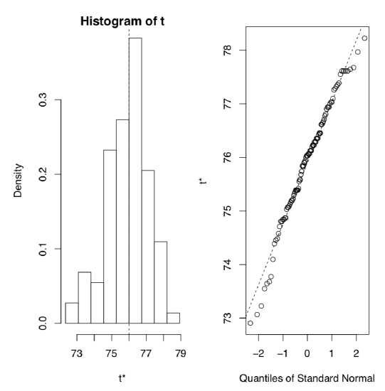
    First, we will bootstrap the mean (Figure \(\PageIndex{2}\)) using the advanced boot package:

    Code \(\PageIndex{1}\) (R):

    library(boot) 
    ## Statistic to be bootstrapped:
    ave.b <- function (data, indices){ 
    d <- data[indices] 
    return(mean(d)) }
    (result.b <- boot(data=trees$Height, statistic=ave.b, R=100))

    (Note that here and in many other places in this book number of replicates is 100. For the working purposes, however, we recommend it to be at least 1,000.)

    Code \(\PageIndex{2}\) (R):

    library(boot)
    ave.b <- function (data, indices){ 
    d <- data[indices] 
    return(mean(d)) }
    result.b <- boot(data=trees$Height, statistic=ave.b, R=100)
    plot(result.b)

    Package boot allows to calculate the 95% confidence interval:

    Code \(\PageIndex{3}\) (R):

    library(boot)
    aave.b <- function (data, indices){ 
    d <- data[indices] 
    return(mean(d)) }
    result.b <- boot(data=trees$Height, statistic=ave.b, R=100)
    boot.ci(result.b, type="bca")

    More basic bootstrap package bootstraps in a simpler way. To demonstrate, we will use the spur.txt data file. This data is a result of measurements of spur length on 1511 Dactylorhiza orchid flowers. The length of spur is important because only pollinators with mouth parts comparable to spur length can successfully pollinate these flowers.

    Code \(\PageIndex{4}\) (R):
    spur <- scan("data/spur.txt")
    library(bootstrap)
    result.b2 <- bootstrap(x=spur, 100, function(x) mean(x))
    ## Median of bootstrapped values:
    median(result.b2$thetastar)
    ## Confidence interval:
    quantile(result.b2$thetastar, probs=c(0.025, 0.975))
    Screen Shot 2019-02-01 at 9.22.11 PM.png Figure \(\PageIndex{2}\) Graphical representation of bootstrapping sample median.

    Jackknife is similar to the bootstrap but in that case observations will be taking out of the sample one by one without replacement:

    Code \(\PageIndex{5}\) (R):

    spur <- scan("data/spur.txt")
    result.j <- jackknife(x=spur, function(x) mean(x))
    ## Median of jackknifed values:
    median(result.j$jack.values)
    ## Standard error:
    result.j$jack.se
    ## Confidence interval:
    quantile(result.j$jack.values, probs=c(0.025, 0.975))

    This is possible to bootstrap standard deviation and mean of this data even without any extra package, with for cycle and sample():

    Code \(\PageIndex{6}\) (R):

    spur <- scan("data/spur.txt")
    boot <- 100
    tt <- matrix(ncol=2, nrow=boot)
    for (n in 1:boot)
    {
    spur.sample <- sample(spur, length(spur), replace=TRUE)
    tt[n, 1] <- mean(spur.sample)
    tt[n, 2] <- sd(spur.sample)
    }
    (result <- data.frame(spur.mean=mean(spur), spur.sd=sd(spur), boot.mean=mean(tt[, 1]), boot.sd=mean(tt[, 2])))

    (Alternatively, tt could be an empty data frame, but this way takes more computer time which is important for bootstrap. What we did above, is the pre-allocation, useful way to save time and memory.)

    Actually, spur length distribution does not follow the normal law (check it yourself). It is better then to estimate median and median absolute deviation (instead of mean and standard deviation), or median and 95% range:

    Code \(\PageIndex{7}\) (R):

    dact <- scan("data/dact.txt")
    quantile(dact, c(0.025, 0.5, 0.975))
    apply(replicate(100, quantile(sample(dact, length(dact), replace=TRUE), c(0.025, 0.5, 0.975))), 1, mean)

    (Note the use of replicate() function, this is another member of apply() family.)

    This approach allows also to bootstrap almost any measures. Let us, for example, bootstrap 95% confidence interval for Lyubishchev’s K:

    Code \(\PageIndex{8}\) (R):

    sleep.K.rep <- replicate(100, K(extra ~ group, data=sleep[sample(1:nrow(sleep), replace=TRUE), ]))
    quantile(sleep.K.rep, c(0.025, 0.975))

    Bootstrap and jackknife are related with numerous resampling techniques. There are multiple R packages (like coin) providing resampling tests and related procedures:

    Code \(\PageIndex{9}\) (R):

    library(coin)
    wilcox_test(V1 ~ V2, data=subset(grades, V2 %in% c("A1", "B1")), conf.int=TRUE)

    Bootstrap is also widely used in the machine learning. Above there was an example of Jclust() function from the asmisc.r set. There also are BootA(), BootRF() and BootKNN() to boorstrap non-supervised and supervised results.

    ) plants. Use bootstrap and resampling methods.


    This page titled 1.6.9.3.3: R and Bootstrapping is shared under a Public Domain license and was authored, remixed, and/or curated by Alexey Shipunov.

    • Was this article helpful?