1.6.9.3.5: R and Bayes

Most of statistical test and many methods use “throwing coin” assumption; however long we throw the coin, probability to see the face is always \(frac{1}{2}\).

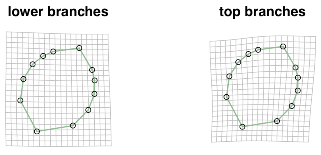
Figure \(\PageIndex{1}\) D’Arcy Thompson’s transformation grids (referenced to the overall mean shape) for alder leaves.

There is another approach, “apple bag”. Suppose we have closed, non-transparent bag full of red and green apples. We took the first apple. It was red. We took the second one. It was red again. Third time: red again. And again.

This means that red apples are likely dominate in the bag. It is because the apple bag is not a coin: it is possible to take all apples from bag and leave it empty but it is impossible to spend all coin throws. Coin throwing is unlimited, apple bag is limited.

So if you like to know proportion of red to green apples in a bag after you took several apples out of it, you need to know some priors: (1) how many apples you took, (2) how many red apples you took, (3) how many apples are in your bag, and then (4) calculate proportions of everything in accordance with particular formula. This formula is a famous Bayes formula but we do not use formulas in this book (except one, and it is already spent).

All in all, Bayesian algorithms use conditional models like our apple bag above. Note that, as with apple bag we need to take apples first and then calculate proportions, in Bayesian algorithms we always need sampling. This is why these algorithms are complicated and were never developed well in pre-computer era.

Below, Bayesian approach exemplified with Bayes factor which in some way is a replacement to p-value.

Whereas p-value approach allows only to reject or fail-to-reject null, Bayes factors allow to express preference (higher degree of belief) towards one of two hypotheses.

If there are two hypotheses, M1 and M2, then Bayes factor of:

< 0 negative (support M2)

0–5 negligible

5–10 substantial

10–15 strong

15–20 very strong

> 20 decisive

So unlike p-value, Bayes factor is also an effect measure, not just a threshold.

To calculate Bayes factor in R, one should be careful because there are plenty of hidden rocks in Bayesian statistics. However, some simple examples will work:

Following is an example of typical two-sample test, traditional and Bayesian:

Code \(\PageIndex{1}\) (R):

## Restrict to two groups
chickwts <- chickwts[chickwts$feed %in% c("horsebean", "linseed"), ]
## Drop unused factor levels
chickwts$feed <- factor(chickwts$feed)
## Plot data
plot(weight ~ feed, data=chickwts, main="Chick weights")
## traditional t test
t.test(weight ~ feed, data=chickwts, var.eq=TRUE)
## Compute Bayes factor
library(BayesFactor)
bf <- ttestBF(formula = weight ~ feed, data=chickwts)
bf

Many more examples are at http://bayesfactorpcl.r-forge.r-project.org/