
10.4 Graphs of Equations
( \newcommand{\kernel}{\mathrm{null}\,}\)
Determining whether a Linear Function Is Increasing, Decreasing, or Constant
The linear functions we used in the two previous examples increased over time, but not every linear function does. A linear function may be increasing, decreasing, or constant. For an increasing function, as with the train example, the output values increase as the input values increase. The graph of an increasing function has a positive slope. A line with a positive slope slants upward from left to right as in Figure 5(a). For a decreasing function, the slope is negative. The output values decrease as the input values increase. A line with a negative slope slants downward from left to right as in Figure 5(b). If the function is constant, the output values are the same for all input values so the slope is zero. A line with a slope of zero is horizontal as in Figure 5(c).
![Three graphs depicting an increasing function, a decreasing function, and a constant function.] Increasing and Decreasing Functions](https://math.libretexts.org/@api/deki/files/13138/CNX_Precalc_Figure_02_01_004abc.jpg?revision=1)
Figure 5: Three graphs depicting an increasing function, a decreasing function, and a constant function.]
Increasing and Decreasing Functions
Increasing and Decreasing Functions
The slope determines if the function is an increasing linear function, a decreasing linear function, or a constant function.
- f(x)=mx+b is an increasing function if m>0.
- f(x)=mx+b is an decreasing function if m<0.
- f(x)=mx+b is a constant function if m=0.
Example 2: Deciding whether a Function Is Increasing, Decreasing, or
Constant
Some recent studies suggest that a teenager sends an average of 60 texts per day. For each of the following scenarios, find the linear function that describes the relationship between the input value and the output value. Then, determine whether the graph of the function is increasing, decreasing, or constant.
a. The total number of texts a teen sends is considered a function of time in days. The input is the number of days, and output is the total number of texts sent.
b. A teen has a limit of 500 texts per month in his or her data plan. The input is the number of days, and output is the total number of texts remaining for the month.
c. A teen has an unlimited number of texts in his or her data plan for a cost of $50 per month. The input is the number of days, and output is the total cost of texting each month.
Solution
Analyze each function.
a. The function can be represented as f(x)=60x where x is the number of days. The slope, 60, is positive so the function is increasing. This makes sense because the total number of texts increases with each day.
b. The function can be represented as f(x)=500−60x where x is the number of days. In this case, the slope is negative so the function is decreasing. This makes sense because the number of texts remaining decreases each day and this function represents the number of texts remaining in the data plan after x days.
c. The cost function can be represented as f(x)=50 because the number of days does not affect the total cost. The slope is 0 so the function is constant.
Calculating and Interpreting Slope
In the examples we have seen so far, we have had the slope provided for us. However, we often need to calculate the slope given input and output values. Given two values for the input, x1 and x2, and two corresponding values for the output, y1 and y2—which can be represented by a set of points, (x1,y1) and (x2,y2)—we can calculate the slope m, as follows
m=change in output (rise)change in input (run)=ΔyΔx=y2−y1x2−x1
where Δy is the vertical displacement and Δx is the horizontal displacement. Note in function notation two corresponding values for the output y1 and y2 for the function f, y1=f(x1) and y2=f(x2), so we could equivalently write
m=f(x2)−f(x1)x2−x1
Figure 6 indicates how the slope of the line between the points, (x1,y1) and (x2,y2), is calculated. Recall that the slope measures steepness. The greater the absolute value of the slope, the steeper the line is.
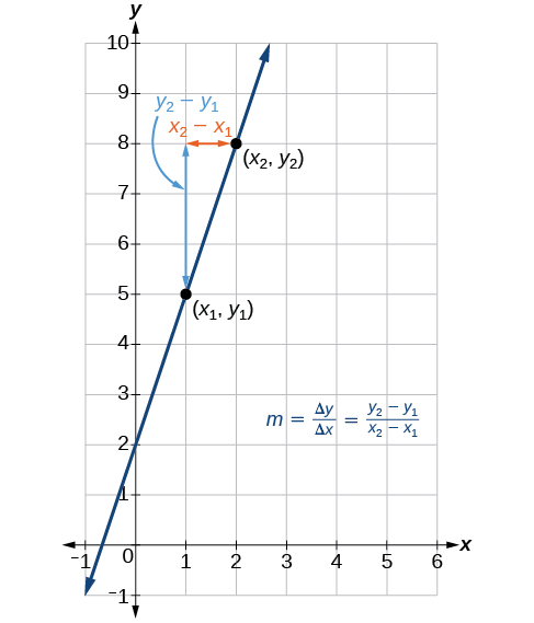
Figure 6: The slope of a function is calculated by the change in y divided by the change in x. It does not matter which coordinate is used as the (x2,y2) and which is the (x1,y1),as long as each calculation is started with the elements from the same coordinate pair.
![]() Are the units for slope always units for the outputunits for the input?
Are the units for slope always units for the outputunits for the input?
Yes. Think of the units as the change of output value for each unit of change in input value. An example of slope could be miles per hour or dollars per day. Notice the units appear as a ratio of units for the output per units for the input.
Calculate Slope
The slope, or rate of change, of a function m can be calculated according to the following:
m=change in output (rise)change in input (run)=ΔyΔx=y2−y1x2−x1
where x1 and x2 are input values, y1 and y2 are output values.
![]() Given two points from a linear function, calculate and interpret the slope.
Given two points from a linear function, calculate and interpret the slope.
- Determine the units for output and input values.
- Calculate the change of output values and change of input values.
- Interpret the slope as the change in output values per unit of the input value.
Example 3: Finding the Slope of a Linear Function
If f(x) is a linear function, and (3,−2) and (8,1) are points on the line, find the slope. Is this function increasing or decreasing?
Solution
The coordinate pairs are (3,−2) and (8,1). To find the rate of change, we divide the change in output by the change in input.
m=change in output (rise)change in input (run)=1−(−2)8−3=35
We could also write the slope as m=0.6. The function is increasing because m>0.
Analysis
As noted earlier, the order in which we write the points does not matter when we compute the slope of the line as long as the first output value, or y-coordinate, used corresponds with the first input value, or x-coordinate, used.
![]() 1: If f(x) is a linear function, and (2,3) and (0,4) are points on the line, find the slope. Is this function increasing or decreasing?
1: If f(x) is a linear function, and (2,3) and (0,4) are points on the line, find the slope. Is this function increasing or decreasing?
Solution
m=4−30−2=1−2=−12; decreasing because m<0.
Writing the Equation of a Line Using a Point and the Slope
The point-slope form is particularly useful if we know one point and the slope of a line. Suppose, for example, we are told that a line has a slope of 2 and passes through the point (4,1). We know that m=2 and that x1=4 and y1=1. We can substitute these values into the general point-slope equation.
y−y1=m(x−x1)y−1=2(x−4)
If we wanted to then rewrite the equation in slope-intercept form, we apply algebraic techniques.
y−1=2(x−4)y−1=2x−8Distribute the 2.y=2x−7Add 1 to each side.
Both equations, y−1=2(x−4) and y=2x–7, describe the same line. See Figure 7.
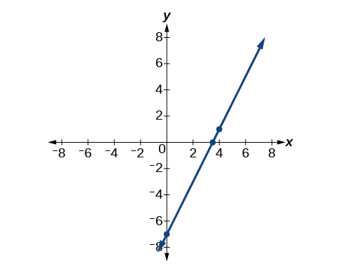
Figure 7
Example 5: Writing Linear Equations Using a Point and the Slope
Write the point-slope form of an equation of a line with a slope of 3 that passes through the point (6,–1). Then rewrite it in the slope-intercept form.
Solution
Let’s figure out what we know from the given information. The slope is 3, so m=3. We also know one point, so we know x1=6 and y1=−1. Now we can substitute these values into the general point-slope equation.
y−y1=m(x−x1)y−(−1)=3(x−6)Substitute known values.y+1=3(x−6)Distribute −1 to find point-slope form.
Then we use algebra to find the slope-intercept form.
y+1=3(x−6)y+1=3x−18Distribute 3.y=3x−19Simplify to slope-intercept form.
![]() 3: Write the point-slope form of an equation of a line with a slope of –2 that passes through the point (–2,2). Then rewrite it in the slope-intercept form.
3: Write the point-slope form of an equation of a line with a slope of –2 that passes through the point (–2,2). Then rewrite it in the slope-intercept form.
Solution
y−2=−2(x+2) ; y=−2x−2