5.7: Area, Volume, and Average Value

Average Value

We know the average of \(n\) numbers \(a_1, a_2, \dots , a_n\) is their sum divided by \(n\). But what if we need to find the average temperature over a day's time – there are too many possible temperatures to add them up! This is a job for the definite integral.

Average Value

The average value of a function \(f(x)\) on the interval \([a, b]\) is given by \[ \frac{1}{b-a}\int_a^bf(x)\, dx. \nonumber \]

The average value of a positive \(f\) has a nice geometric interpretation. Imagine that the area under \(f\) (graph (a) below) is a liquid that can leak through the graph to form a rectangle with the same area (graph (b) below).

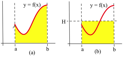
If the height of the rectangle is \(H\), then the area of the rectangle is \( H\cdot (b-a) \). We know the area of the rectangle is the same as the area under \(f\) so \( H\cdot (b-a) = \int_a^b f(x)\, dx \). Then \[ H = \frac{1}{b-a}\int_a^b f(x)\, dx, \nonumber \] the average value of \(f\) on \([a,b]\).

The average value of a positive function \(f\) is the height \(H\) of the rectangle whose area is the same as the area under \(f\).

Example \(\PageIndex{1}\)

During a 9 hour work day, the production rate at time \(t\) hours after the start of the shift was given by the function \( r(t)=5+\sqrt{t} \) cars per hour. Find the average hourly production rate.

Solution

The average hourly production is \( \frac{1}{9-0}\int_0^9\left(5+\sqrt{t}\right)\, dt = 7 \) cars per hour.

A note about the units – remember that the definite integral has units (cars per hour)\( \cdot \)(hours) = cars. But the \( \frac{1}{b-a} \) in front has units \(\frac{1}{\text{hours}}\) so the units of the average value are cars per hour, just what we expect an average rate to be.

In general...

…the average value of a function will have the same units as the integrand.

Function averages, involving means and more complicated averages, are used to smooth data so that underlying patterns are more obvious and to remove high frequency noise from signals. In these situations, the original function \(f\) is replaced by some average of \(f\). If \(f\) is rather jagged time data, then the ten year average of \(f\) is the integral \( g(x)=\frac{1}{10}\int\limits_{x-5}^{x+5} f(t)\, dt \), an average of \(f\) over 5 units on each side of \(x\).

For example, the figure below shows the graphs of a Monthly Average (rather “noisy” data) of surface temperature data, an Annual Average (still rather jagged), and a Five Year Average (a much smoother function).

Image prepared by Robert A. Rohde, http://commons.wikimedia.org/wiki/File:Short_Instrumental_Temperature_Record.png.

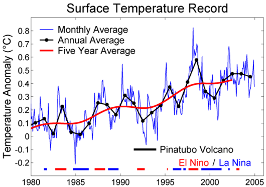
Typically the average function reveals the pattern much more clearly than the original data. This use of a moving average value of noisy data (weather information, stock prices) is a very common.

Example \(\PageIndex{2}\)

The graph below shows the amount of water in a reservoir over a 12 hour period. Estimate the average amount of water in the reservoir over this period.

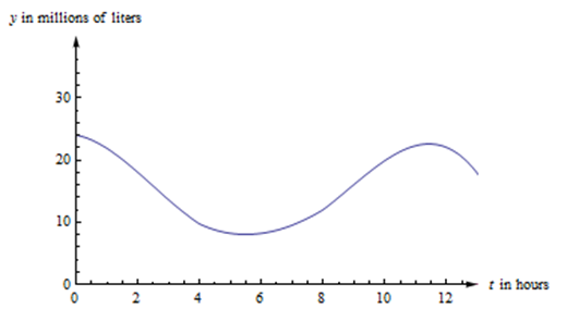
If \( V(t) \) is the volume of the water (in millions of liters) after \(t\) hours, then the average amount is \( \frac{1}{12}\,\int_0^{12} V(t)\, dt \). In order to find the definite integral, we'll have to estimate. Let's use 6 rectangles and take the heights from their right edges (there's nothing special about using 6 rectangles or right edges – other choices would still give you a valid estimate).

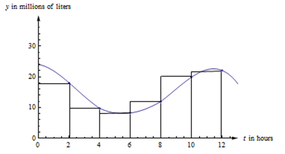
The estimate of the integral is \[\int_0^{12} V(t)\, dt \approx (18)(2)+(9.7)(2)+(8.2)(2)+(12)(2)+(19.9)(2)+(22)(2)=179.6.\nonumber \]

Solution

The units of this integral are (millions of liters)\( \cdot \)(feet). So our estimate of the average volume is \( \frac{1}{12}\cdot 179.6\approx 15 \) millions of liters. (The estimate might change a little depending on how we estimate the function values from the graph.)

In the figure below, you can see the same graph with the line \( y=15 \) drawn in. The area under the curve and the area under the rectangle are (approximately) the same.

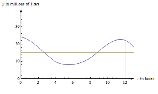
In fact, that would be a different way to estimate the average value. We could have estimated the placement of the horizontal line so that the area under the curve and under the line were equal.

Area

We have already used integrals to find the area between the graph of a function and the horizontal axis. Integrals can also be used to find the area between two graphs.

If \(f(x) \geq g(x)\) for all \(x\) in \([a,b]\), then we can approximate the area between \(f\) and \(g\) by partitioning the interval \([a,b]\) and forming a Riemann sum, as shown in the picture. The height of each rectangle is top - bottom, \(f(c_i) - g(c_i)\) so the area of the \(i\)-th rectangle is (height)\( \cdot \)(base) = \(\left(f(c_i) - g(c_i)\right)\cdot\Delta x\). Adding up these rectangles gives an approximation of the total area as \( \sum_{i=1}^n \left(f(c_i) - g(c_i)\right)\cdot\Delta x \), a Riemann sum.

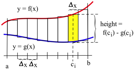
The limit of this Riemann sum, as the number of rectangles gets larger and their width gets smaller, is the definite integral \( \int_a^b \left(f(x) - g(x)\right)\, dx \).

Area Between Two Curves

The area between two curves \(f(x)\) and \(g(x)\), where \(f(x) \geq g(x)\), between \(x = a\) and \(x = b\) is \[ \int_a^b \left(f(x) - g(x)\right)\, dx. \nonumber \]

The integrand is top - bottom. Make a graph or use test values to be sure which curve is which.

Example \(\PageIndex{3}\)

Find the area bounded between the graphs of \(f(x) = x\) and \(g(x) = 3\) for \(1 \leq x \leq 4\).

Solution

Always start with a graph so you can see which graph is the top and which is the bottom. In this example, the two curves cross, and they change positions; we’ll need to split the area into two pieces. Geometrically, we can see that the area is 2 + 0.5 = 2.5.

Writing the area as a sum of definite integrals, we get \[ \text{Area }= \int_1^3 (3-x)\, dx+\int_3^4 (x-3)\, dx.\nonumber \]

These integrals are easy to evaluate using antiderivatives: \[ \begin{align*} \int_1^3 (3-x)\, dx & = \left[3x-\frac{x^2}{2}\right]_1^3 \\ & = \left(9-\frac{9}{2}\right)-\left(3-\frac{1}{2}\right) \\ & = 2 \end{align*} \nonumber \] \[ \begin{align*} \int_3^4 (x-3)\, dx & = \left[\frac{x^2}{2}-3x\right]_3^4 \\ & = \left(\frac{16}{2}-12\right)-\left(\frac{9}{2}-9\right) \\ & = \frac{1}{2} \end{align*} \nonumber \]

The sum of these two integrals tells us that the total area between \(f\) and \(g\) is 2.5 square units, which we already knew from the picture.

Note that the single integral \( \int_1^4 (3-x)\, dx = 1.5 \) is not the area we want in the last example. The value of the integral is 1.5, and the value of the area is 2.5. That's because for the triangle on the right, the graph of \(y = x\) is above the graph of \(y = 3\), so the integrand \(3 - x\) is negative; in the definite integral, the area of that triangle comes in with a negative sign.

In this example, it was easy to see exactly where the two curves crossed so we could break the region into the two pieces to figure separately. In other examples, you might need to solve an equation to find where the curves cross.

Example \(\PageIndex{4}\)

Find the area bounded by the graphs of \(f(x) = x^2\) and \(g(x) = x+6\).

Solution

To begin, it will help to sketch a graph of the functions to see the area enclosed.

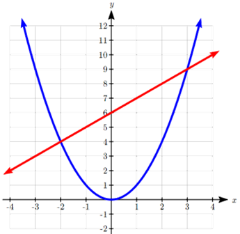
To set up the integral for the area, we need to determine where the line intersects the parabola. While the points look fairly clear in the graph, it will be good to verify the points algebraically: \[ \begin{align*} x^2 & = x+6 \\ x^2 - x -6 & = 0 \\ (x-3)(x+2) & = 1 \\ x & = -2, 3 \end{align*} \nonumber \]

Over this interval \(-2 \leq x \le 3\) notice the linear function is on top, so if we were to draw a rectangle between the curves, the height would be (top function) − (bottom function) = \((x+6)-x^2\).

Setting up a definite integral for this area: \[ \text{Area }= \int_{-2}^3 (x+6-x^2)\, dx\nonumber \]

We can evaluate this integral using antiderivatives: \[ \begin{align*} \int_{-2}^3 (x+6-x^2)\, dx & = \left[\frac{x^2}{2} + 6x - \frac{x^3}{3}\right]_{-2}^3 \\ & = \left(\frac{3^2}{2} + 6\cdot 3 -\frac{3^3}{3}\right)-\left(\frac{(-2)^2}{2} + 6\cdot(-2) -\frac{(-2)^3}{3}\right) \\ & = \left(\frac{9}{2} + 18 - \frac{27}{3}\right) - \left(\frac{4}{2} - 12 +\frac{8}{3}\right) \\ & = \left(\frac{9}{2} + 18 - 9\right) - \left(2 - 12 +\frac{8}{3}\right) \\ & = \left(\frac{9}{2} +9\right) - \left(-10 +\frac{8}{3}\right) \\ & = \frac{9}{2} +9 +10 -\frac{8}{3} \\ & = \frac{125}{6} \end{align*} \nonumber \]

The area between the curves is \(\frac{125}{6}\approx 20.833\) square units.

Example \(\PageIndex{5}\)

Two objects start from the same location and travel along the same path with velocities \( v_A(t)=t+3 \) and \( v_B(t)=t^2-4t+3 \) meters per second. How far ahead is \(A\) after 3 seconds?

Solution

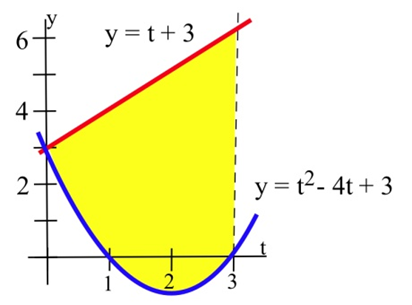
Since \( v_A(t) \geq v_B(t) \), the area between the graphs of \( v_A \) and \( v_B \) represents the distance between the objects.

After 3 seconds, the distance apart is \[ \begin{align*} \int_0^3 \left( v_A(t) - v_B(t) \right)\, dt & = \int_0^3 \left( (t+3) - \left( t^2-4t+3 \right) \right)\, dt \\ & = \int_0^3 \left(5t-t^2\right)\, dt \\ & = \left[ 5\frac{t^2}{2} -\frac{t^3}{3} \right]_0^3 \\ & = \left( 5\frac{9}{2}-\frac{27}{3}\right)-(0) \\ & = 13.5 \text{ meters}. \end{align*} \nonumber \]

Volume

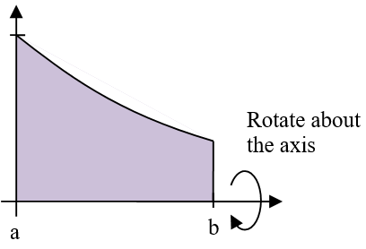
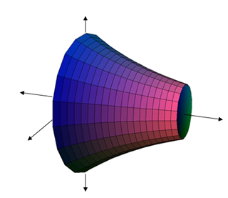
Just as we can partition an interval and imagine approximating an area with rectangles to find a formula for the area between curves, we can partition an interval and imagine approximating a volume with simple shapes to find a formula for the volume of a solid. While this approach works for a variety of shapes, our focus will be on shapes formed by revolving a curve around the horizontal axis.

We start with an area, the region below a function on the interval \(a \leq x \leq b\). We are going to take that region, and rotate it around the \(x\)-axis, creating the solid shape shown.

To find the volume of this solid, we can start by partitioning the interval [0,1] and approximating the area with rectangles. As before, the width of each rectangle would be \( \Delta x \) and the height \(f(c_i)\).

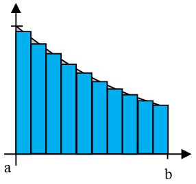
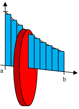
If we took just one of these rectangles and rotated it about the horizontal axis, it would form a cylindrical shape. The radius of that cylinder would be \(f(c_i)\), so the volume would be \[ V=\pi r^2 h=\pi\left(f(c_i)\right)^2\Delta x. \nonumber \]

The volume of the whole solid could be approximated by rotating each of the rectangles about the x axis. Adding up the volume of each of the little cylindrical discs gives an approximation of the total volume as \( \sum\limits_{i=1}^n \pi\left(f(c_i)\right)^2\Delta x \), a Riemann sum.

The limit of this sum as the width of the rectanges becomes small is the definite integral \( \int_a^b \pi\left(f(c_i)\right)^2\, dx \)

Volume

The volume of the solid obtained by rotating about the \(x\)-axis the area bounded by the curve \(f(x)\), the \(x\)-axis, \(x = a\), and \(x = b\) is \[ \int_a^b \pi\left(f(c_i)\right)^2\, dx \nonumber \]

Example \(\PageIndex{6}\)

Find the volume of the solid formed by rotating the area under \( f(x)=e^{-x} \) on the interval [0,1] about the \(x\)-axis.

Solution

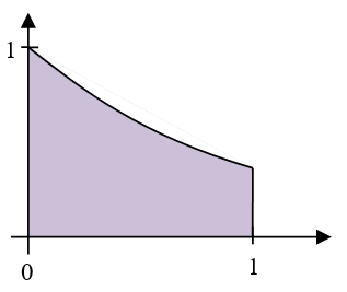
This is the region pictured in the earlier example. We substitute in the function and bounds into the formula we derived to set up the definite integral: \[ \text{Volume} = \int_0^1 \pi\left(e^{-x}\right)^2\, dx. \nonumber \]

Using exponent rules, the integrand can be simplified. The constant \( \pi \) can be pulled out of the integral: \[ \text{Volume} = \pi\int_0^1 e^{-2x}\, dx. \nonumber \]

Using the substitution \(u = -2x\), we can integrate this function. \[ \begin{align*} \pi\int_0^1 e^{-2x}\, dx & = \text{(\( u \)-substitution)} \\ & = \left. -\frac{1}{2}\pi e^{-2x}\right]_0^1 \\ & = \left(-\frac{1}{2}\pi e^{-2(1)}\right) - \left(-\frac{1}{2}\pi e^{-2(0)}\right) \\ \approx & 1.358\text{ cubic units}. \end{align*} \nonumber \]