1.1: Review of Functions

Learning Objectives

• Use functional notation to evaluate a function.
• Determine the domain and range of a function.
• Draw the graph of a line.
• Find function values from a given graph.
• Use a graph to determine where a function is increasing, decreasing, or constant.
• Make new functions from composing given functions.
• Find the difference quotient of a function.

In this section, we provide a formal definition of a function and examine several ways in which functions are represented—namely, through tables, formulas, and graphs. We study formal notation and terms related to functions. We also define composition of functions and symmetry properties. Most of this material will be a review for you, but it serves as a handy reference to remind you of some of the algebraic techniques useful for working with functions.

Functions

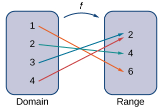
Given two sets $A$ and $B$ a set with elements that are ordered pairs $(x,y)$ where $x$ is an element of $A$ and $y$ is an element of $B,$ is a relation from $A$ to $B$. A relation from $A$ to $B$ defines a relationship between those two sets. A function is a special type of relation in which each element of the first set is related to exactly one element of the second set. The element of the first set is called the input; the element of the second set is called the output. Functions are used all the time in mathematics to describe relationships between two sets. For any function, when we know the input, the output is determined, so we say that the output is a function of the input. For example, the area of a square is determined by its side length, so we say that the area (the output) is a function of its side length (the input). The velocity of a ball thrown in the air can be described as a function of the amount of time the ball is in the air. The cost of mailing a package is a function of the weight of the package. Since functions have so many uses, it is important to have precise definitions and terminology to study them.

Figure $\PageIndex{1}$: A function can be visualized as an input/output device

Definition: Functions

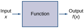
A function $f$ consists of a set of inputs, a set of outputs, and a rule for assigning each input to exactly one output. The set of inputs is called the domain of the function. The set of outputs is called the range of the function.

Figure $\PageIndex{2}$: A function maps every element in the domain to exactly one element in the range. Although each input can be sent to only one output, two different inputs can be sent to the same output.

For example, consider the function $f$, where the domain is the set of all real numbers and the rule is to square the input. Then, the input $x=3$ is assigned to the output $3^2=9$.

Since every nonnegative real number has a real-value square root, every nonnegative number is an element of the range of this function. Since there is no real number with a square that is negative, the negative real numbers are not elements of the range. We conclude that the range is the set of nonnegative real numbers.

For a general function $f$ with domain $D$, we often use $x$ to denote the input and $y$ to denote the output associated with $x$. When doing so, we refer to $x$ as the independent variable and $y$ as the dependent variable, because it depends on $x$. Using function notation, we write $y=f(x)$, and we read this equation as “$y$ equals $f$ of $x.”$ For the squaring function described earlier, we write $f(x)=x^2$.

The concept of a function can be visualized using Figures $\PageIndex{1}$ - $\PageIndex{3}$.

Figure $\PageIndex{3}$: In this case, a graph of a function $f$ has a domain of $\{1,2,3\}$ and a range of $\{1,2\}$. The independent variable is $x$ and the dependent variable is $y$.

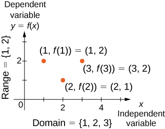
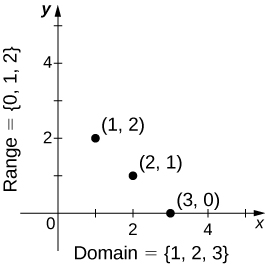
We can also visualize a function by plotting points $(x,y)$ in the coordinate plane where $y=f(x)$. The graph of a function is the set of all these points. For example, consider the function $f$, where the domain is the set $D=\{1,2,3\}$ and the rule is $f(x)=3−x$. In Figure $\PageIndex{4}$, we plot a graph of this function.

Figure $\PageIndex{4}$: Here we see a graph of the function $f$ with domain $\{1,2,3\}$ and rule $f(x)=3−x$. The graph consists of the points $(x,f(x))$ for all $x$ in the domain.

Every function has a domain. However, sometimes a function is described by an equation, as in $f(x)=x^2$, with no specific domain given. In this case, the domain is taken to be the set of all real numbers $x$ for which $f(x)$ is a real number. For example, since any real number can be squared, if no other domain is specified, we consider the domain of $f(x)=x^2$ to be the set of all real numbers. On the other hand, the square root function $f(x)=\sqrt{x}$ only gives a real output if $x$ is nonnegative. Therefore, the domain of the function $f(x)=\sqrt{x}$ is the set of nonnegative real numbers, sometimes called the natural domain.

For the functions $f(x)=x^2$ and $f(x)=\sqrt{x}$, the domains are sets with an infinite number of elements. Clearly we cannot list all these elements. When describing a set with an infinite number of elements, it is often helpful to use set-builder or interval notation. When using set-builder notation to describe a subset of all real numbers, denoted $R$, we write

$$\{x\,|\,\textit{x has some property}\}. \nonumber$$

We read this as the set of real numbers $x$ such that $x$ has some property. For example, if we were interested in the set of real numbers that are greater than one but less than five, we could denote this set using set-builder notation by writing

$$\{x\,|\,1<x<5\}.\nonumber$$

A set such as this, which contains all numbers greater than $a$ and less than $b,$ can also be denoted using the interval notation $(a,b)$. Therefore,

$$(1,5)=\{x\,|\,1<x<5\}.\nonumber$$

The numbers $1$ and $5$ are called the endpoints of this set. If we want to consider the set that includes the endpoints, we would denote this set by writing

$$[1,5]=\{x\,|\,1 \le x \le 5\}.\nonumber$$

We can use similar notation if we want to include one of the endpoints, but not the other. To denote the set of nonnegative real numbers, we would use the set-builder notation

$$\{x\,|\,x\ge 0\}.\nonumber$$

The smallest number in this set is zero, but this set does not have a largest number. Using interval notation, we would use the symbol $∞,$ which refers to positive infinity, and we would write the set as

$$[0,∞)=\{x\,|\,x\ge 0\}.\nonumber$$

It is important to note that $∞$ is not a real number. It is used symbolically here to indicate that this set includes all real numbers greater than or equal to zero. Similarly, if we wanted to describe the set of all nonpositive numbers, we could write

$$(−∞,0]=\{x\,|\,x≤0\}.\nonumber$$

Here, the notation $−∞$ refers to negative infinity, and it indicates that we are including all numbers less than or equal to zero, no matter how small. The set

$$(−∞,∞)=\{\textit{x} \,|\, \textit{x is any real number}\}\nonumber$$

refers to the set of all real numbers. Some functions are defined using different equations for different parts of their domain. These types of functions are known as piecewise-defined functions. For example, suppose we want to define a function $f$ with a domain that is the set of all real numbers such that $f(x)=3x+1$ for $x≥2$ and $f(x)=x^2$ for $x<2$. We denote this function by writing

$$f(x)=\begin{cases} 3x+1, & \text{if } x≥2 \\ x^2, & \text{if } x<2 \end{cases}\nonumber$$

When evaluating this function for an input $x$, the equation to use depends on whether $x≥2$ or $x<2$. For example, since $5>2$, we use the fact that $f(x)=3x+1$ for $x≥2$ and see that $f(5)=3(5)+1=16$. On the other hand, for $x=−1$, we use the fact that $f(x)=x^2$ for $x<2$ and see that $f(−1)=1$.

Example $\PageIndex{1}$: Evaluating Functions

For the function $f(x)=3x^2+2x−1$, evaluate:

1. $f(−2)$
2. $f(\sqrt{2})$
3. $f(a+h)$

Solution

Substitute the given value for $x$ in the formula for $f(x)$.

1. $f(−2)=3(−2)^2+2(−2)−1=12−4−1=7$
2. $f(\sqrt{2})=3(\sqrt{2})^2+2\sqrt{2}−1=6+2\sqrt{2}−1=5+2\sqrt{2}$
3. $f(a+h)=3(a+h)^2+2(a+h)−1=3(a^2+2ah+h^2)+2a+2h−1=3a^2+6ah+3h^2+2a+2h−1$

Exercise $\PageIndex{1}$

For $f(x)=x^2−3x+5$, evaluate $f(1)$ and $f(a+h)$.

Hint

Substitute $1$ and $a+h$ for $x$ in the formula for $f(x)$.

Answer

$f(1)=3$ and $f(a+h)=a^2+2ah+h^2−3a−3h+5$

Example $\PageIndex{2}$: Finding Domain and Range

For each of the following functions, determine the i. domain and ii. range.

1. $f(x)=(x−4)^2+5$
2. $f(x)=\sqrt{3x+2}−1$
3. $f(x)=\dfrac{3}{x−2}$

Solution

a. Consider $f(x)=(x−4)^2+5.$

1.Since $f(x)=(x−4)^2+5$ is a real number for any real number $x$, the domain of $f$ is the interval $(−∞,∞)$.

2. Since $(x−4)^2≥0$, we know $f(x)=(x−4)^2+5≥5$. Therefore, the range must be a subset of $\{y\,|\,y≥5\}.$ To show that every element in this set is in the range, we need to show that for a given $y$ in that set, there is a real number $x$ such that $f(x)=(x−4)^2+5=y$. Solving this equation for $x,$ we see that we need $x$ such that

$(x−4)^2=y−5.$

This equation is satisfied as long as there exists a real number $x$ such that

$x−4=±\sqrt{y−5}$

Since $y≥5$, the square root is well-defined. We conclude that for $x=4±\sqrt{y−5},$ $f(x)=y,$ and therefore the range is $\{y\,|\,y≥5 \}.$

b. Consider $f(x)=\sqrt{3x+2}−1$.

1.To find the domain of $f$, we need the expression $3x+2≥0$. Solving this inequality, we conclude that the domain is $\{x\,|\,x≥−2/3\}.$

2.To find the range of $f$, we note that since $\sqrt{3x+2}≥0,$ $f(x)=\sqrt{3x+2}−1≥−1$. Therefore, the range of $f$ must be a subset of the set $\{y\,|\,y≥−1\}$. To show that every element in this set is in the range of $f$, we need to show that for all $y$ in this set, there exists a real number $x$ in the domain such that $f(x)=y.$ Let $y≥−1.$ Then, $f(x)=y$ if and only if

$\sqrt{3x+2}−1=y.$

Solving this equation for $x,$ we see that $x$ must solve the equation

$\sqrt{3x+2}=y+1.$

Since $y≥−1$, such an $x$ could exist. Squaring both sides of this equation, we have $3x+2=(y+1)^2.$

Therefore, we need

$3x=(y+1)^2−2,$

which implies

$x=\frac{1}{3}(y+1)^2−\frac{2}{3}.$

We just need to verify that $x$ is in the domain of $f$. Since the domain of $f$ consists of all real numbers greater than or equal to $\frac{−2}{3}$, and

$\frac{1}{3}(y+1)^2-\frac{2}{3}≥−\frac{2}{3},$

there does exist an $x$ in the domain of $f$. We conclude that the range of $f$ is $\{y\,|\,y≥−1\}.$

c. Consider $f(x)=\dfrac{3}{x−2}.$

1.Since $3/(x−2)$ is defined when the denominator is nonzero, the domain is $\{x\,|\,x≠2\}.$

2.To find the range of $f,$ we need to find the values of $y$ such that there exists a real number $x$ in the domain with the property that

$\dfrac{3}{x−2}=y.$

Solving this equation for $x,$ we find that

$x=\dfrac{3}{y}+2.$

Therefore, as long as $y≠0$, there exists a real number $x$ in the domain such that $f(x)=y$. Thus, the range is $\{y\,|\,y≠0\}.$

Exercise $\PageIndex{2}$

Find the domain and range for $f(x)=\sqrt{4−2x}+5.$

Hint

Use $4−2x≥0$.

Answer

Domain = $\{x\,|\,x≤2\}$ and range = $\{y\,|\,y≥5\}$

Finding Function Values from a Graph

Evaluating a function using a graph also requires finding the corresponding output value for a given input value, only in this case, we find the output value by looking at the graph. Solving a function equation using a graph requires finding all instances of the given output value on the graph and observing the corresponding input value(s).

Example $\PageIndex{3}$: Reading Function Values from a Graph

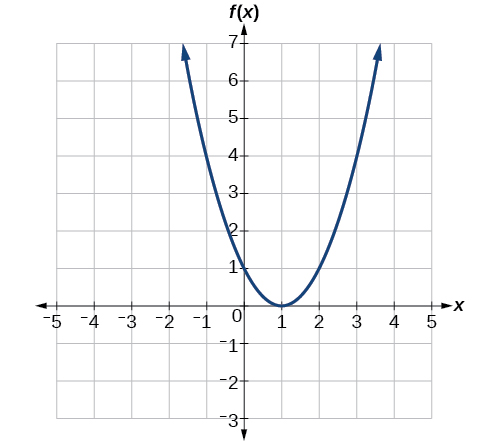
Given the graph in Figure $\PageIndex{7}$,

1. Evaluate $f(2)$.
2. Solve $f(x)=4$.

Figure $\PageIndex{7}$: Graph of a positive parabola centered at $(1, 0)$.

Solution

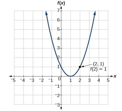
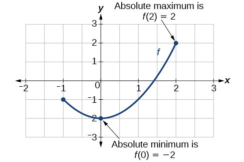
To evaluate $f(2)$, locate the point on the curve where $x=2$, then read the y-coordinate of that point. The point has coordinates $(2,1)$, so $f(2)=1$. See Figure $\PageIndex{8}$.

$\PageIndex{8}$: Graph of a positive parabola centered at $(1, 0)$ with the labeled point $(2, 1)$ where $f(2) =1$.

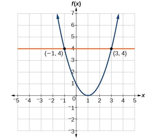
To solve $f(x)=4$, we find the output value 4 on the vertical axis. Moving horizontally along the line $y=4$, we locate two points of the curve with output value 4: $(−1,4)$ and $(3,4)$. These points represent the two solutions to $f(x)=4$: −1 or 3. This means $f(−1)=4$ and $f(3)=4$, or when the input is −1 or 3, the output is 4. See Figure $\PageIndex{9}$.

Figure $\PageIndex{9}$: Graph of an upward-facing parabola with a vertex at $(0,1)$ and labeled points at $(-1, 4)$ and $(3,4)$. A line at $y = 4$ intersects the parabola at the labeled points.

Exercise $\PageIndex{3}$

Given the graph in Figure $\PageIndex{7}$, solve $f(x)=1$.

Answer

$x=0$ or $x=2$

Using a Graph to Determine Where a Function is Increasing, Decreasing, or Constant

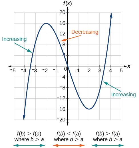
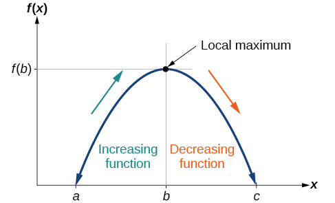
As part of exploring how functions change, we can identify intervals over which the function is changing in specific ways. We say that a function is increasing on an interval if the function values increase as the input values increase within that interval. Similarly, a function is decreasing on an interval if the function values decrease as the input values increase over that interval. The average rate of change of an increasing function is positive, and the average rate of change of a decreasing function is negative. Figure $\PageIndex{3}$ shows examples of increasing and decreasing intervals on a function.

Figure $\PageIndex{3}$: The function $f(x)=x^3−12x$ is increasing on $(−\infty, −2)\cup (2,\infty)$ and is decreasing on $(−2, 2)$.

While some functions are increasing (or decreasing) over their entire domain, many others are not. A value of the input where a function changes from increasing to decreasing (as we go from left to right, that is, as the input variable increases) is called a local maximum. If a function has more than one, we say it has local maxima. Similarly, a value of the input where a function changes from decreasing to increasing as the input variable increases is called a local minimum. The plural form is “local minima.” Together, local maxima and minima are called local extrema, or local extreme values, of the function. (The singular form is “extremum.”) Often, the term local is replaced by the term relative. In this text, we will use the term local.

Clearly, a function is neither increasing nor decreasing on an interval where it is constant. A function is also neither increasing nor decreasing at extrema. Note that we have to speak of local extrema, because any given local extremum as defined here is not necessarily the highest maximum or lowest minimum in the function’s entire domain.

For the function whose graph is shown in Figure $\PageIndex{4}$, the local maximum is 16, and it occurs at $x=−2$. The local minimum is −16 and it occurs at $x=2$.

Figure $\PageIndex{4}$: Graph of a polynomial that shows the increasing and decreasing intervals and local maximum.maximum

To locate the local maxima and minima from a graph, we need to observe the graph to determine where the graph attains its highest and lowest points, respectively, within an open interval. Like the summit of a roller coaster, the graph of a function is higher at a local maximum than at nearby points on both sides. The graph will also be lower at a local minimum than at neighboring points. Figure $\PageIndex{5}$ illustrates these ideas for a local maximum.

Figure $\PageIndex{5}$: Definition of a local maximum

These observations lead us to a formal definition of local extrema.

Local Minima and Local Maxima

• A function $f$ is an increasing function on an open interval if $f(b)>f(a)$ for every $a$, $b$ interval where $b>a$.
• A function $f$ is a decreasing function on an open interval if $f(b)<f(a)$ for every $a$, $b$ interval where $b>a$.

A function $f$ has a local maximum at a point $b$ in an open interval $(a,c)$ if $f(b)$ is greater than or equal to $f(x)$ for every point $x$ ($x$ does not equal $b$) in the interval. Likewise, $f$ has a local minimum at a point $b$ in $(a,c)$ if $f(b)$ is less than or equal to $f(x)$ for every $x$ ($x$ does not equal $b$) in the interval.

Example $\PageIndex{4}$ Finding Increasing and Decreasing Intervals on a Graph

Given the function $p(t)$ in Figure $\PageIndex{6}$, identify the intervals on which the function appears to be increasing.

Figure $\PageIndex{6}$: Graph of a polynomial.

Solution

We see that the function is not constant on any interval. The function is increasing where it slants upward as we move to the right and decreasing where it slants downward as we move to the right. The function appears to be increasing from $t=1$ to $t=3$ and from $t=4$ on.

In interval notation, we would say the function appears to be increasing on the interval $(1,3)$ and the interval $(4,\infty)$.

Analysis

Notice in this example that we used open intervals (intervals that do not include the endpoints), because the function is neither increasing nor decreasing at $t=1$, $t=3$, and $t=4$. These points are the local extrema (two minima and a maximum).

Example $\PageIndex{5}$: Finding Local Extrema from a Graph

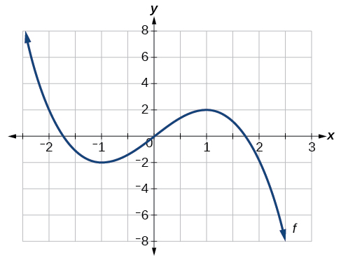
Graph the function $f(x)=\frac{2}{x}+\frac{x}{3}$. Then use the graph to estimate the local extrema of the function and to determine the intervals on which the function is increasing.

Solution

Using technology, we find that the graph of the function looks like that in Figure $\PageIndex{7}$. It appears there is a low point, or local minimum, between $x=2$ and $x=3$, and a mirror-image high point, or local maximum, somewhere between $x=−3$ and $x=−2$

.

Figure $\PageIndex{7}$: Graph of a reciprocal function.

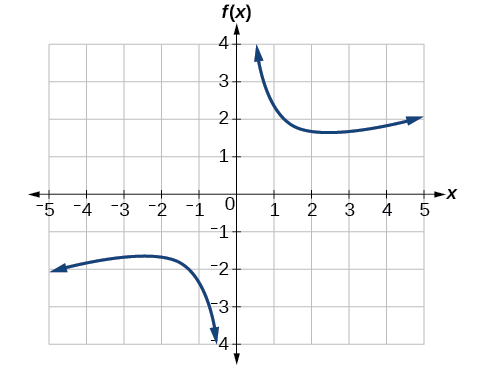Analysis

Most graphing calculators and graphing utilities can estimate the location of maxima and minima. Figure $\PageIndex{8}$ provides screen images from two different technologies, showing the estimate for the local maximum and minimum.

Figure $\PageIndex{8}$: Graph of the reciprocal function on a graphing calculator.

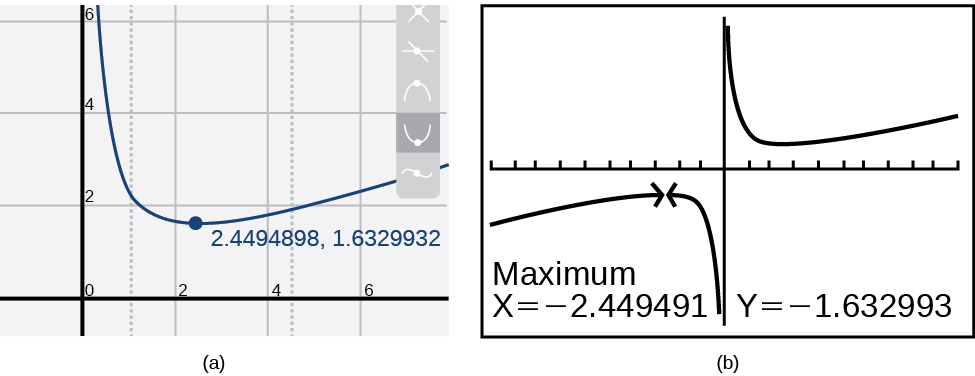
Based on these estimates, the function is increasing on the interval $(−\infty,−2.449)$ and $(2.449,\infty)$. Notice that, while we expect the extrema to be symmetric, the two different technologies agree only up to four decimals due to the differing approximation algorithms used by each. (The exact location of the extrema is at $\pm\sqrt{6}$, but determining this requires calculus.)

Exercise $\PageIndex{5}$

Graph the function $f(x)=x^3−6x^2−15x+20$ to estimate the local extrema of the function. Use these to determine the intervals on which the function is increasing and decreasing.

Solution

The local maximum appears to occur at $(−1,28)$, and the local minimum occurs at $(5,−80)$. The function is increasing on $(−\infty,−1)\cup(5,\infty)$ and decreasing on $(−1,5)$.

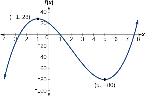
Graph of a polynomial with a local maximum at (-1, 28) and local minimum at (5, -80).

Example $\PageIndex{6}$: Finding Local Maxima and Minima from a Graph

For the function f whose graph is shown in Figure $\PageIndex{9}$, find all local maxima and minima.

Figure $\PageIndex{9}$: Graph of a polynomial.

Solution

Observe the graph of $f$. The graph attains a local maximum at $x=1$ because it is the highest point in an open interval around $x=1$.The local maximum is the y-coordinate at $x=1$, which is 2.

The graph attains a local minimum at $x=−1$ because it is the lowest point in an open interval around $x=−1$. The local minimum is the y-coordinate at $x=−1$, which is −2.

Use A Graph to Locate the Absolute Maximum and Absolute Minimum

There is a difference between locating the highest and lowest points on a graph in a region around an open interval (locally) and locating the highest and lowest points on the graph for the entire domain. The y-coordinates (output) at the highest and lowest points are called the absolute maximum and absolute minimum, respectively. To locate absolute maxima and minima from a graph, we need to observe the graph to determine where the graph attains it highest and lowest points on the domain of the function (Figure $\PageIndex{13}$).

Figure $\PageIndex{13}$: Graph of a segment of a parabola with an absolute minimum at (0, -2) and absolute maximum at (2, 2).

Not every function has an absolute maximum or minimum value. The toolkit function $f(x)=x^3$ is one such function.

Absolute Maxima and Minima

• The absolute maximum of $f$ at $x=c$ is $f(c)$ where $f(c)≥f(x)$ for all $x$ in the domain of $f$.
• The absolute minimum of $f$ at $x=d$ is $f(d)$ where $f(d)≤f(x)$ for all $x$ in the domain of $f$.

Example $\PageIndex{7}$: Finding Absolute Maxima and Minima from a Graph

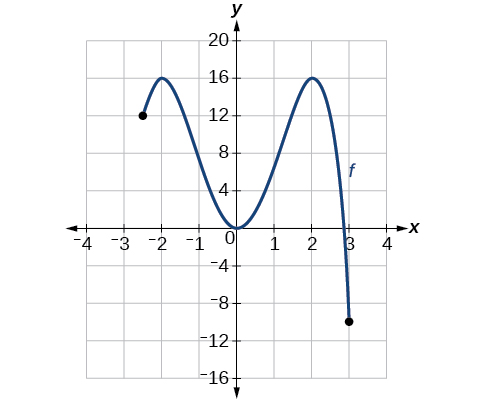
For the function f shown in Figure $\PageIndex{14}$, find all absolute maxima and minima.

Figure $\PageIndex{14}$: Graph of a polynomial.

Solution

Observe the graph of $f$. The graph attains an absolute maximum in two locations, $x=−2$ and $x=2$, because at these locations, the graph attains its highest point on the domain of the function. The absolute maximum is the y-coordinate at $x=−2$ and $x=2$, which is 16.

The graph attains an absolute minimum at x=3, because it is the lowest point on the domain of the function’s graph. The absolute minimum is the y-coordinate at x=3,which is−10.

Function Composition

When we compose functions, we take a function of a function. For example, suppose the temperature $T$ on a given day is described as a function of time $t$ (measured in hours after midnight) as in Table $\PageIndex{1}$. Suppose the cost $C$, to heat or cool a building for 1 hour, can be described as a function of the temperature $T$. Combining these two functions, we can describe the cost of heating or cooling a building as a function of time by evaluating $C(T(t))$. We have defined a new function, denoted $C∘T$, which is defined such that $(C∘T)(t)=C(T(t))$ for all $t$ in the domain of $T$. This new function is called a composite function. We note that since cost is a function of temperature and temperature is a function of time, it makes sense to define this new function $(C∘T)(t)$. It does not make sense to consider $(T∘C)(t)$, because temperature is not a function of cost.

Definition: Composite Functions

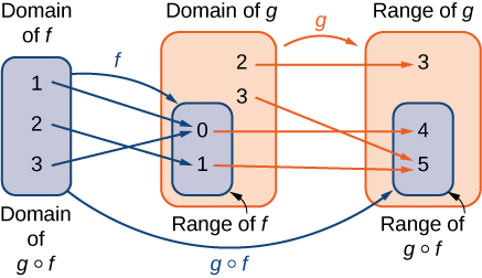
Consider the function $f$ with domain $A$ and range $B$, and the function $g$ with domain $D$ and range $E$. If $B$ is a subset of $D$, then the composite function $(g∘f)(x)$ is the function with domain $A$ such that

$$(g∘f)(x)=g(f(x)) \nonumber$$

A composite function $g∘f$ can be viewed in two steps. First, the function $f$ maps each input $x$ in the domain of $f$ to its output $f(x)$ in the range of $f$. Second, since the range of $f$ is a subset of the domain of $g$, the output $f(x)$ is an element in the domain of $g$, and therefore it is mapped to an output $g(f(x))$ in the range of $g$. In Figure $\PageIndex{11}$, we see a visual image of a composite function.

Figure $\PageIndex{11}$: For the composite function $g∘f$, we have $(g∘f)(1)=4,$ $(g∘f)(2)=5,$ and $(g∘f)(3)=4$.

Example $\PageIndex{7}$: Compositions of Functions Defined by Formulas

Consider the functions $f(x)=x^2+1$ and $g(x)=1/x$.

1. Find $(g∘f)(x)$ and state its domain and range.
2. Evaluate $(g∘f)(4),$ $(g∘f)(−1/2)$.
3. Find $(f∘g)(x)$ and state its domain and range.
4. Evaluate $(f∘g)(4),$ $(f∘g)(−1/2)$.

Solution

1. We can find the formula for $(g∘f)(x)$ in two different ways. We could write

$(g∘f)(x)=g(f(x))=g(x^2+1)=\dfrac{1}{x^2+1}$.

Alternatively, we could write

$(g∘f)(x)=g(f(x))=\dfrac{1}{f(x)}=\dfrac{1}{x^2+1}.$

Since $x^2+1≠0$ for all real numbers $x,$ the domain of $(g∘f)(x)$ is the set of all real numbers. Since $0<1/(x^2+1)≤1$, the range is, at most, the interval $(0,1]$. To show that the range is this entire interval, we let $y=1/(x^2+1)$ and solve this equation for $x$ to show that for all $y$ in the interval $(0,1]$, there exists a real number $x$ such that $y=1/(x^2+1)$. Solving this equation for $x,$ we see that $x^2+1=1/y$, which implies that

$x=±\sqrt{\frac{1}{y}−1}$

If $y$ is in the interval $(0,1]$, the expression under the radical is nonnegative, and therefore there exists a real number $x$ such that $1/(x^2+1)=y$. We conclude that the range of $g∘f$ is the interval $(0,1].$

2. $(g∘f)(4)=g(f(4))=g(4^2+1)=g(17)=\frac{1}{17}$

$(g∘f)(−\frac{1}{2})=g(f(−\frac{1}{2}))=g((−\frac{1}{2})^2+1)=g(\frac{5}{4})=\frac{4}{5}$

3. We can find a formula for $(f∘g)(x)$ in two ways. First, we could write

$(f∘g)(x)=f(g(x))=f(\frac{1}{x})=(\frac{1}{x})^2+1.$

Alternatively, we could write

$(f∘g)(x)=f(g(x))=(g(x))^2+1=(\frac{1}{x})^2+1.$

The domain of $f∘g$ is the set of all real numbers $x$ such that $x≠0$. To find the range of $f,$ we need to find all values $y$ for which there exists a real number $x≠0$ such that

$\left(\dfrac{1}{x}\right)^2+1=y.$

Solving this equation for $x,$ we see that we need $x$ to satisfy

$\left(\dfrac{1}{x}\right)^2=y−1,$

which simplifies to

$\dfrac{1}{x}=±\sqrt{y−1}$

Finally, we obtain

$x=±\dfrac{1}{\sqrt{y−1}}.$

Since $1/\sqrt{y−1}$ is a real number if and only if $y>1,$ the range of $f$ is the set $\{y\,|\,y≥1\}.$

4.$(f∘g)(4)=f(g(4))=f(\frac{1}{4})=(\frac{1}{4})^2+1=\frac{17}{16}$

$(f∘g)(−\frac{1}{2})=f(g(−\frac{1}{2}))=f(−2)=(−2)^2+1=5$

In Example $\PageIndex{7}$, we can see that $(f∘g)(x)≠(g∘f)(x)$. This tells us, in general terms, that the order in which we compose functions matters.

Exercise $\PageIndex{7}$

Let $f(x)=2−5x$. Let $g(x)=\sqrt{x}.$ Find $(f∘g)(x)$.

Solution

$(f∘g)(x)=2−5\sqrt{x}.$

Example $\PageIndex{8}$: Composition of Functions Defined by Tables

Consider the functions $f$ and $g$ described by

$x$	-3	-2	-1	0	1	2	3	4
$f(x)$	0	4	2	4	-2	0	-2	4

$x$	-4	-2	0	2	4
$g(x)$	1	0	3	0	5

1. Evaluate $(g∘f)(3)$,$(g∘f)(0)$.
2. State the domain and range of $(g∘f)(x)$.
3. Evaluate $(f∘f)(3)$,$(f∘f)(1)$.
4. State the domain and range of $(f∘f)(x)$.

Solution:

1. $(g∘f)(3)=g(f(3))=g(−2)=0$

$(g∘f)(0)=g(4)=5$

2.The domain of $g∘f$ is the set $\{−3,−2,−1,0,1,2,3,4\}.$ Since the range of $f$ is the set $\{−2,0,2,4\},$ the range of $g∘f$ is the set $\{0,3,5\}.$

3. $(f∘f)(3)=f(f(3))=f(−2)=4$

$(f∘f)(1)=f(f(1))=f(−2)=4$

4.The domain of $f∘f$ is the set $\{−3,−2,−1,0,1,2,3,4\}.$ Since the range of $f$ is the set $\{−2,0,2,4\},$ the range of $f∘f$ is the set $\{0,4\}.$

Example $\PageIndex{9}$: Application Involving a Composite Function

A store is advertising a sale of 20% off all merchandise. Caroline has a coupon that entitles her to an additional 15% off any item, including sale merchandise. If Caroline decides to purchase an item with an original price of $x$ dollars, how much will she end up paying if she applies her coupon to the sale price? Solve this problem by using a composite function.

Solution

Since the sale price is 20% off the original price, if an item is $x$ dollars, its sale price is given by $f(x)=0.80x$. Since the coupon entitles an individual to 15% off the price of any item, if an item is $y$ dollars, the price, after applying the coupon, is given by g(y)=0.85y. Therefore, if the price is originally $x$ dollars, its sale price will be $f(x)=0.80x$ and then its final price after the coupon will be $g(f(x))=0.85(0.80x)=0.68x$.

Exercise $\PageIndex{9}$

If items are on sale for 10% off their original price, and a customer has a coupon for an additional 30% off, what will be the final price for an item that is originally $x$ dollars, after applying the coupon to the sale price?

Hint

The sale price of an item with an original price of $x$ dollars is $f(x)=0.90x$. The coupon price for an item that is $y$ dollars is $g(y)=0.70y$.

Solution

$(g∘f)(x)=0.63x$

The Difference Quotient

Let’s imagine a point on the curve of function $f$ at x as shown in Figure 13. The coordinates of the point are $\left(x,f\left(x\right)\right)$. Connect this point with a second point on the curve a little to the right of $x$, with an x-value increased by some small real number $h$. The coordinates of this second point are $\left(x+h,f\left(x+h\right)\right)$ for some positive-value $h$.

Figure $\PageIndex{12}$: Connecting point $a$ with a point just beyond allows us to measure a slope close to that of a tangent line at x.

We can calculate the slope of the line connecting the two points $\left(x,f\left(x\right)\right)$ and $\left(x+h,f\left(x+h\right)\right)$, called a secant line, by applying the slope formula,

$\text{slope = }\dfrac{\text{change in }y}{\text{change in }x}$

$\text{slope = }\dfrac{\text{change in }y}{\text{change in }x}$

We use the notation ${m}_{\sec }$ to represent the slope of the secant line connecting two points.

$$\begin{align}{m}_{\sec }&=\dfrac{f\left(x+h\right)-f\left(x\right)}{\left(x+h\right)-\left(x\right)} \\ &=\dfrac{f\left(x+h\right)-f\left(x\right)}{h} \end{align}$$

The slope ${m}_{\sec }$ equals the difference quotient between two points $\left(x,f\left(x\right)\right)$ and $\left(x+h,f\left(x+h\right)\right)$.

Definition: The Difference Quotient

The difference quotient between two points $\left(x,f\left(x\right)\right)$ and $\left(x+h,f\left(x+h\right)\right)$ on the curve of $f$ is the slope of the line connecting the two points and is given by

$\text{difference quotient}=\dfrac{f\left(x+h\right)-f\left(x\right)}{h}$

Example $\PageIndex{10}$: Finding the difference quotient (Quadratic function)

Find the difference quotient if $(x)=2x^{2}-x$.

Solution

We use the difference quotient formula.

​ $$\begin{align}\frac{f\left(x+h\right)-f\left(x\right)}{h}\hspace{.5in} & \text{Start with the difference quotient} \\ \frac{2(x+h)^{2}-(x+h)-(2x^{2}-x)}{h}\hspace{.5in} & \text{Replace x with (x+h)} \\ \frac{2(x^{2}+2xh+h^{2})-x-h-2x^{2}+x}{h}\hspace{.5in} & \text{Distribute} \\ \frac{2x^2+4xh+2h^2-x-h-2x^2+x}{h}\hspace{.5in} & \text{Distribute} \\ \frac{4xh+2h^{2}-h}{h}\hspace{.5in} & \text{Simplify like terms} \\ 4x+2h-1\hspace{.5in} & \text{This is the difference quotient}\end{align}$$

Exercise $\PageIndex{10}$

Find the difference quotient if $f\left(x\right)={x}^{2}+2x - 8$.

Answer

$2x+h+2$

Example $\PageIndex{11}$: Finding the difference quotient (Rational function)

Find the difference quotient if $f(x)=\dfrac{1}{x}$.

Solution

We use the difference quotient formula.

$$\begin{align}\dfrac{f\left(x+h\right)-f\left(x\right)}{h}\hspace{.5in} & \text{Start with the difference quotient} \\ \dfrac{\dfrac{1}{x+h}-\dfrac{1}{x}}{h}\hspace{.5in} & \text{Replace x with (x+h)} \\ \dfrac{\dfrac{x}{x(x+h)}-\dfrac{x+h}{x(x+h)}}{h}\hspace{.5in} & \text{Get common denominators} \\ \dfrac{\dfrac{x-x-h}{x(x+h)}}{h}\hspace{.5in} & \text{Subtract the fractions} \\ \dfrac{-h}{x(x+h)h}\hspace{.5in} & \text{Flip and multiply} \\ \dfrac{-1}{x(x+h)}\hspace{.5in} & \text{This is the difference quotient}\end{align}$$

Exercise $\PageIndex{11}$

Find the difference quotient if $f(x)=-\dfrac{2}{x}$.

Answer

$\dfrac{2}{x(x+h)}$