2.2: Graphing the Basic Functions

Learning Objectives

• Define and graph seven basic functions.
• Define and graph piecewise functions.
• Evaluate piecewise defined functions.

Prerequisite Skills

Before you get started, take this prerequisite quiz.

1. Simplify \((-3)^2\) without using a calculator.

Click here to check your answer

\(9\)

If you missed this problem, review here. (Note that this will open a different textbook in a new window.)

 

2. Simplify \((-3)^3\) without using a calculator.

Click here to check your answer

\(-27\)

If you missed this problem, review here. (Note that this will open a different textbook in a new window.)

 

3. Simplify \(|-3|\).

Click here to check your answer

\(3\)

If you missed this problem, review here. (Note that this will open a different textbook in a new window.)

 

4. Simplify \(\sqrt{4}\).

Click here to check your answer

\(2\) 

If you missed this problem, review here. (Note that this will open a different textbook in a new window.)

 

5. Simplify \(\dfrac{1}{1/3}\).

Click here to check your answer

\(3\) 

If you missed this problem, review here. (Note that this will open a different textbook in a new window.)

 

6. On a piece of graph paper, plot and label these points: A(3, -1), B(-2, -4), C(0, 0), D(-4, 0), E(0, 3).

Click here to check your answer

 

If you missed this problem, review here. (Note that this will open a different textbook in a new window.)

Basic Functions

In this section we graph seven basic functions that will be used throughout this course. Each function is graphed by plotting points. Remember that \(f (x) = y\) and thus \(f (x)\) and \(y\) can be used interchangeably.

Any function of the form \(f (x) = c\), where \(c\) is any real number, is called a constant function⁴³. Constant functions are linear and can be written \(f (x) = 0x + c\). In this form, it is clear that the slope is \(0\) and the \(y\)-intercept is \((0, c)\). Evaluating any value for \(x\), such as \(x = 2\), will result in \(c\).

Figure 2.4.1

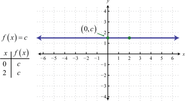
The graph of a constant function is a horizontal line. The domain is \((-\infty,\infty)\) and the range consists of the single value \(\{c\}\).

We next define the identity function⁴⁴ \(f (x) = x\). Evaluating any value for \(x\) will result in that same value. For example, \(f (0) = 0\) and \(f (2) = 2\). The identity function is linear, \(f (x) = 1x + 0\), with slope \(m = 1\) and \(y\)-intercept \((0, 0)\).

Figure 2.4.2

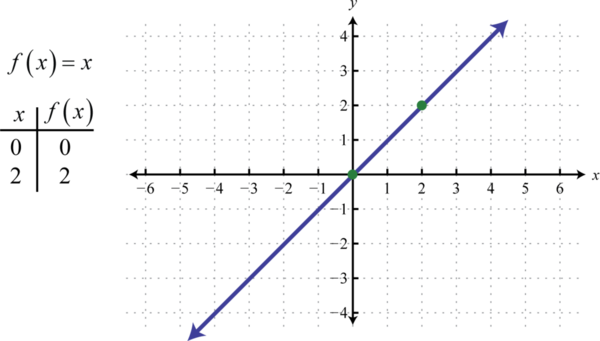
The domain and range both consist of all real numbers, \((-\infty,\infty)\).

The squaring function⁴⁵, defined by \(f (x) = x^{2}\), is the function obtained by squaring the values in the domain. For example, \(f (2) = (2)^{2} = 4\) and \(f (−2) = (−2)^{2} = 4\).The result of squaring nonzero values in the domain will always be positive.

Figure 2.4.3

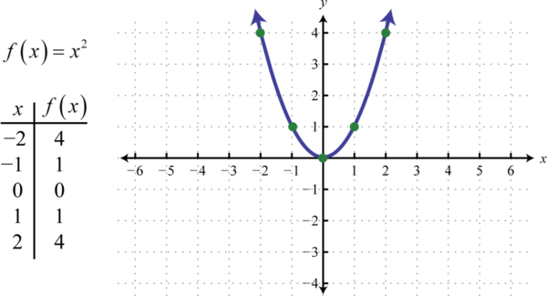
The resulting curved graph is called a parabola⁴⁶. The domain is \((-\infty,\infty)\) and the range is \([0, ∞)\).  We will look at parabolas more in depth in Section 2.4.

The cubing function⁴⁷, defined by \(f (x) = x^{3}\), raises all of the values in the domain to the third power. The results can be either negative, zero, or positive. For example, \(f (-1) = (-1)^{3} = -1, f (0) = (0)^{3} = 0\), and \(f (1) = (1)^{3} = 1\).

Figure 2.4.4

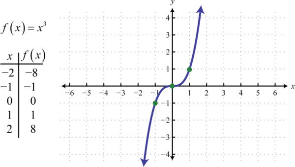
The domain and range both consist of all real numbers, \((-\infty,\infty)\).

Note that the constant, identity, squaring, and cubing functions are all examples of basic polynomial functions. The next three basic functions are not polynomials.

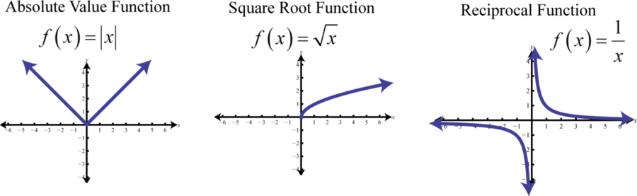
The absolute value function⁴⁸, defined by \(f (x) = |x|\), is a function where the output represents the distance to the origin on a number line. The result of evaluating the absolute value function for any nonzero value of \(x\) will always be positive. For example, \(f (−2) = |−2| = 2\) and \(f (2) = |2| = 2\).

Figure 2.4.5

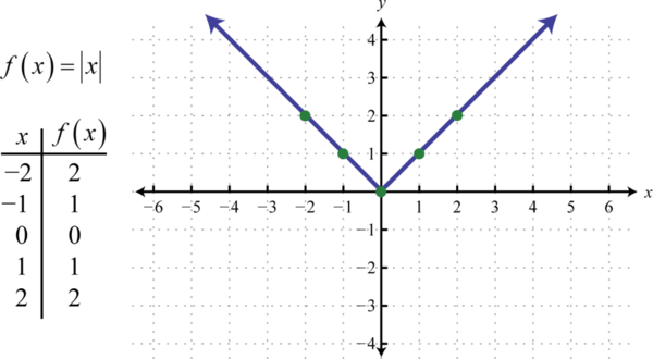
Like the parabola, the domain is \((-\infty,\infty)\) and the range is \([0, ∞)\).

The square root function⁴⁹, defined by \(f (x) = \sqrt{x}\), is not defined to be a real number if the \(x\)-values are negative. Therefore, the smallest value in the domain is zero. For example, \(f (0) = \sqrt{0}= 0\) and \(f (4) = \sqrt{4}= 2\).

Figure 2.4.6

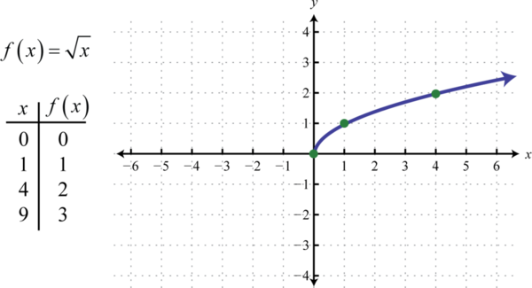
The domain and range both consist of real numbers greater than or equal to zero \([0, ∞)\).

The reciprocal function⁵⁰, defined by \(f (x) = \frac{1}{x}\), is a rational function with one restriction on the domain, namely \(x ≠ 0\). The reciprocal of an \(x\)-value very close to zero is very large. For example,

\(\begin{aligned} f ( 1 / 10 ) &= \frac { 1 } { \left( \frac { 1 } { 10 } \right) } = 1 \cdot \frac { 10 } { 1 } = 10 \\ f ( 1 / 100 ) &= \frac { 1 } { \left( \frac { 1 } { 100 } \right) } = 1 \cdot \frac { 100 } { 1 } = 100 \\ f ( 1 / 1,000 )& = \frac { 1 } { \left( \frac { 1 } { 1,000 } \right) } = 1 \cdot \frac { 1,000 } { 1 } = 1,000 \end{aligned}\)

In other words, as the \(x\)-values approach zero their reciprocals will tend toward either positive or negative infinity. This describes a vertical asymptote⁵¹ at the \(y\)-axis. Furthermore, where the \(x\)-values are very large the result of the reciprocal function is very small.

\(\begin{aligned} f ( 10 ) & = \frac { 1 } { 10 } = 0.1 \\ f ( 100 ) & = \frac { 1 } { 100 } = 0.01 \\ f ( 1000 ) & = \frac { 1 } { 1,000 } = 0.001 \end{aligned}\)

In other words, as the \(x\)-values become very large the resulting \(y\)-values tend toward zero. This describes a horizontal asymptote⁵² at the \(x\)-axis. After plotting a number of points the general shape of the reciprocal function can be determined.

Figure 2.4.7

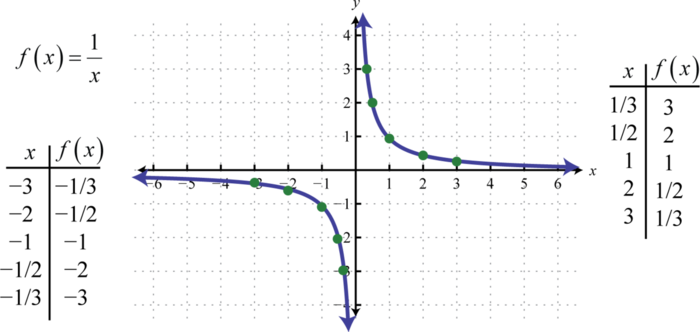
Both the domain and range of the reciprocal function consists of all real numbers except \(0\),or \((−∞, 0) ∪ (0, ∞)\).  We will look at the reciprocal function more in depth in Section 2.6.

In summary, the basic polynomial functions are:

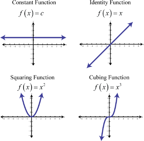
Figure 2.4.8

The basic nonpolynomial functions are:

Figure 2.4.9

Piecewise Defined Functions

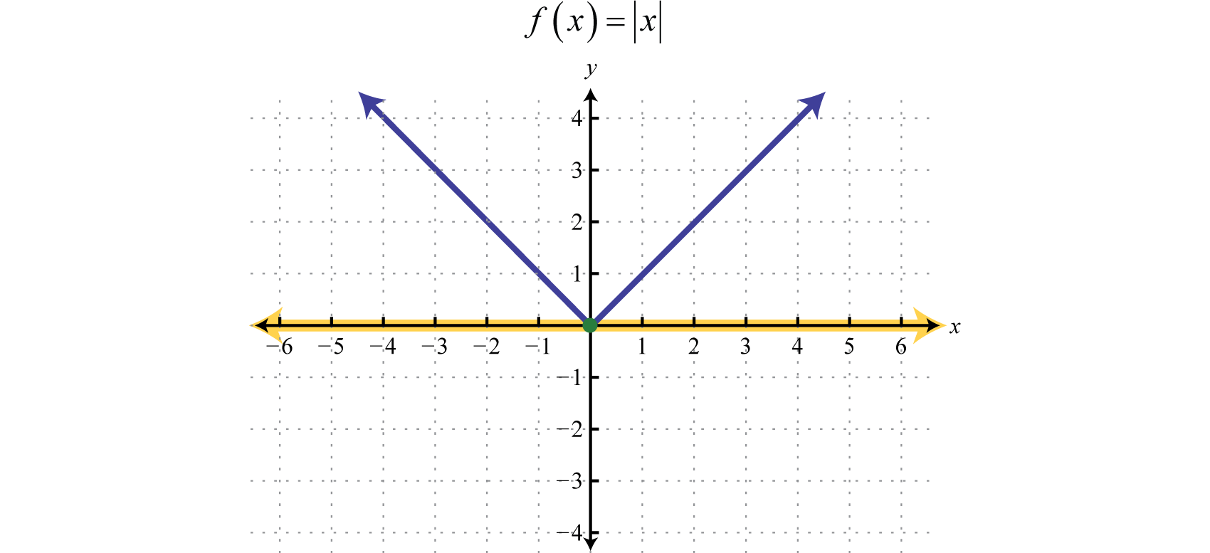
A piecewise function⁵³, or split function⁵⁴, is a function whose definition changes depending on the value in the domain. For example, we can write the absolute value function \(f(x) = |x|\) as a piecewise function:

\(f ( x ) = | x | = \left\{ \begin{array} { c l } { x } & { \text { if } x \geq 0 } \\ { - x } & { \text { if } x < 0 } \end{array} \right.\)

In this case, the definition used depends on the sign of the \(x\)-value. If the \(x\)-value is positive, \(x ≥ 0\), then the function is defined by \(f(x) = x\). And if the \(x\)-value is negative, \(x < 0\), then the function is defined by \(f(x) = −x\).

Figure 2.4.10

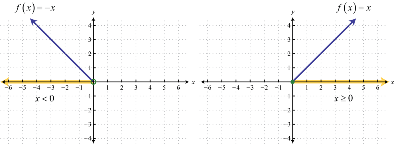
Following is the graph of the two pieces on the same rectangular coordinate plane:

Figure 2.4.11

Example \(\PageIndex{1}\):

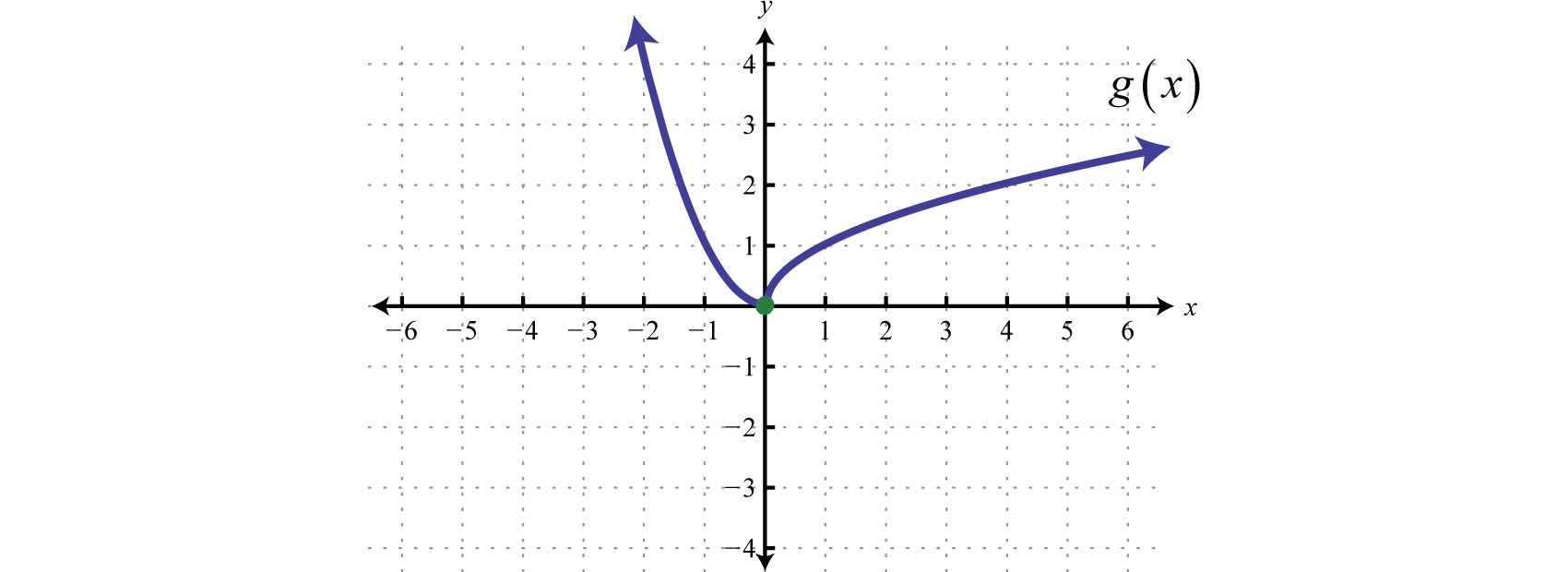
Graph: \(g ( x ) = \left\{ \begin{array} { c c c } { x ^ { 2 } } & { \text { if } } & { x < 0 } \\ { \sqrt { x } } & { \text { if } } & { x \geq 0 } \end{array} \right.\).

Solution

In this case, we graph the squaring function over negative \(x\)-values and the square root function over positive \(x\)-values.

Figure 2.4.12

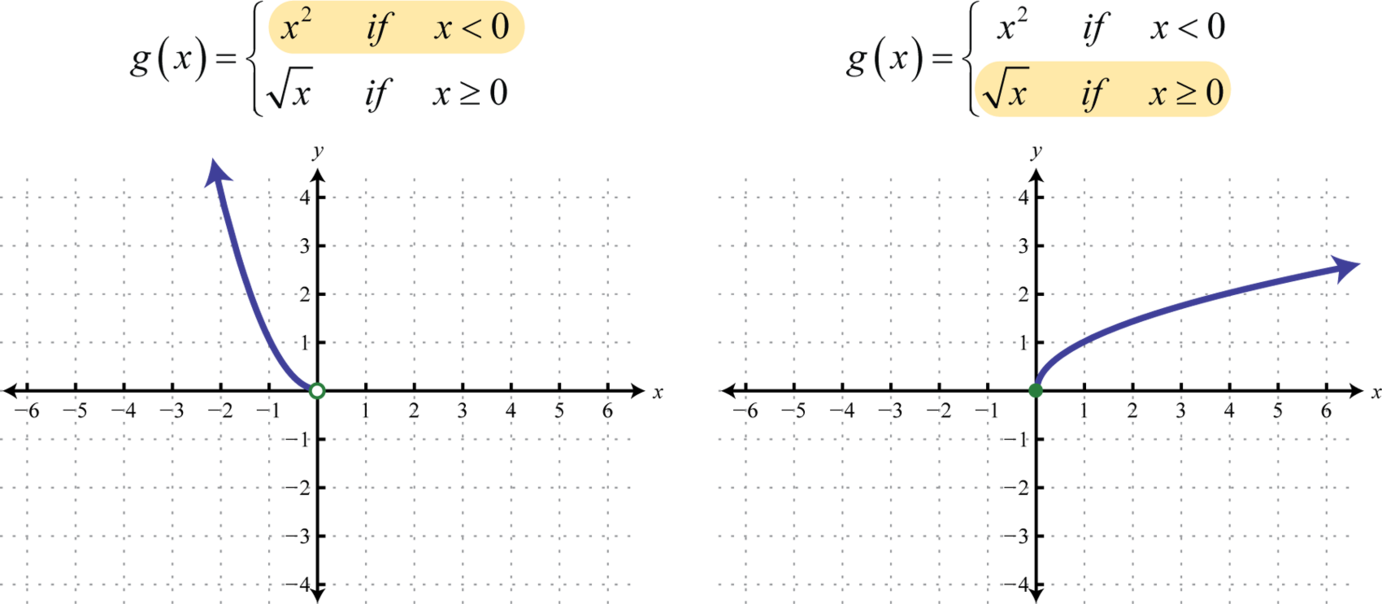
Notice the open dot used at the origin for the squaring function and the closed dot used for the square root function. This was determined by the inequality that defines the domain of each piece of the function. The entire function consists of each piece graphed on the same coordinate plane.

Answer:

Figure 2.4.13

When evaluating, the value in the domain determines the appropriate definition to use.

Example \(\PageIndex{2}\):

Given the function \(h ( t ) = \left\{ \begin{array} { l l } { 7t + 3 } & { \text { if } t < 0 } \\ { −16t^{2} + 32t } & { \text { if } t \geq 0 } \end{array} \right.\), find \(h(−5), h(0),\) and \(h(3)\).

Solution

Use \(h(t) = 7t + 3\) where \(t\) is negative, as indicated by \(t < 0\).

\(\begin{aligned} h ( t ) & = 7 t + 5 \\ h ( \color{Cerulean}{- 5}\color{Black}{ )} & = 7 ( \color{Cerulean}{- 5}\color{Black}{)} + 3 \\ & = - 35 + 3 \\ & = - 32 \end{aligned}\)

Where \(t\) is greater than or equal to zero, use \(h(t) = −16t^{2} + 32t\).

\(\begin{aligned} h ( \color{Cerulean}{0}\color{Black}{ )} & = - 16 ( \color{Cerulean}{0}\color{Black}{ )} + 32 ( \color{Cerulean}{0}\color{Black}{ )} \text {  and  }  h ( \color{Cerulean}{3}\color{Black}{ )} = 16 ( \color{Cerulean}{3}\color{Black}{ )} ^ { 2 } + 32 ( \color{Cerulean}{3}\color{Black}{ )} \\ & = 0 + 0 \quad\quad\quad\quad\quad\:\quad = -144 +96 \\ & = 0 \quad\quad\quad\quad\quad\quad\quad\quad = - 48 \end{aligned}\)

Answer:

\(h(−5) = −32, h(0) = 0,\) and \(h(3) = −48\)

Exercise \(\PageIndex{1}\)

Graph: \(f ( x ) = \left\{ \begin{array} { l l } { \frac { 2 } { 3 } x + 1 } & { \text { if } x < 0 } \\ { x ^ { 2 } } & { \text { if } x \geq 0 } \end{array} \right.\).

Answer

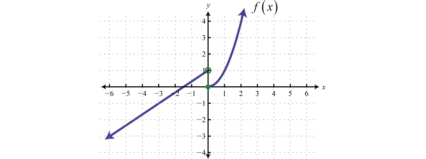
Figure 2.4.14

www.youtube.com/v/0hEUnSN5Blw

The definition of a function may be different over multiple intervals in the domain.

Example \(\PageIndex{3}\):

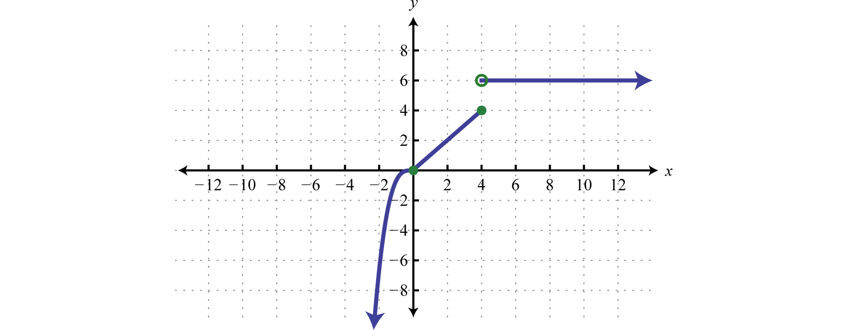
Graph: \(f ( x ) = \left\{ \begin{array} { l l } { x ^ { 3 } } & { \text { if } x < 0 } \\ { x } & { \text { if } 0 \leq x \leq 4 } \\ { 6 } & { \text { if } x > 4 } \end{array} \right.\).

Solution

In this case, graph the cubing function over the interval \((−∞,0)\). Graph the identity function over the interval \([0,4]\). Finally, graph the constant function \(f(x)=6\) over the interval \((4,∞)\). And because \(f(x)=6\) where \(x>4\), we use an open dot at the point \((4,6)\). Where \(x=4\), we use \(f(x)=x\) and thus \((4,4)\) is a point on the graph as indicated by a closed dot.

Answer:

Figure 2.4.15

 

Key Takeaways

• Plot points to determine the general shape of the basic functions. The shape, as well as the domain and range, of each should be memorized.
• The basic polynomial functions are: \(f(x) = c, f(x) = x , f(x) = x^{2}\), and \(f(x) = x^{3}\).
• The basic nonpolynomial functions are: \(f(x) = |x|, f(x) = \sqrt{x}\), and \(f(x) = \frac{1}{x}\).
• A function whose definition changes depending on the value in the domain is called a piecewise function. The value in the domain determines the appropriate definition to use.

Footnotes

⁴³Any function of the form \(f(x) = c\) where \(c\) is a real number.

⁴⁴The linear function defined by \(f(x) = x\).

⁴⁵The quadratic function defined by \(f(x) = x^{2}\).

⁴⁶The curved graph formed by the squaring function.

⁴⁷The cubic function defined by \(f(x) = x^{3}\).

⁴⁸The function defined by \(f(x) = |x|\).

⁴⁹The function defined by \(f(x) = \sqrt{x}\).

⁵⁰The function defined by \(f(x) = \frac{1}{x}\).

⁵¹A vertical line to which a graph becomes infinitely close.

⁵²A horizontal line to which a graph becomes infinitely close where the \(x\)-values tend toward \(±∞\).

⁵³A function whose definition changes depending on the values in the domain.

⁵⁴A term used when referring to a piecewise function.

⁵⁵The function that assigns any real number \(x\) to the greatest integer less than or equal to \(x\) denoted \(f(x) = \left[\!\![x]\!\!\right]\).

⁵⁶A term used when referring to the greatest integer function.