2.5: Polynomial Functions

Last updated
Save as PDF

Page ID: 48337

$ \newcommand{\vecs}[1]{\overset { \scriptstyle \rightharpoonup} {\mathbf{#1}} } $

$ \newcommand{\vecd}[1]{\overset{-\!-\!\rightharpoonup}{\vphantom{a}\smash {#1}}} $

$ \newcommand{\id}{\mathrm{id}}$ $ \newcommand{\Span}{\mathrm{span}}$

( \newcommand{\kernel}{\mathrm{null}\,}\) $ \newcommand{\range}{\mathrm{range}\,}$

$ \newcommand{\RealPart}{\mathrm{Re}}$ $ \newcommand{\ImaginaryPart}{\mathrm{Im}}$

$ \newcommand{\Argument}{\mathrm{Arg}}$ $ \newcommand{\norm}[1]{\| #1 \|}$

$ \newcommand{\inner}[2]{\langle #1, #2 \rangle}$

$ \newcommand{\Span}{\mathrm{span}}$

$ \newcommand{\id}{\mathrm{id}}$

$ \newcommand{\Span}{\mathrm{span}}$

$ \newcommand{\kernel}{\mathrm{null}\,}$

$ \newcommand{\range}{\mathrm{range}\,}$

$ \newcommand{\RealPart}{\mathrm{Re}}$

$ \newcommand{\ImaginaryPart}{\mathrm{Im}}$

$ \newcommand{\Argument}{\mathrm{Arg}}$

$ \newcommand{\norm}[1]{\| #1 \|}$

$ \newcommand{\inner}[2]{\langle #1, #2 \rangle}$

$ \newcommand{\Span}{\mathrm{span}}$ $ \newcommand{\AA}{\unicode[.8,0]{x212B}}$

$ \newcommand{\vectorA}[1]{\vec{#1}} % arrow$

$ \newcommand{\vectorAt}[1]{\vec{\text{#1}}} % arrow$

$ \newcommand{\vectorB}[1]{\overset { \scriptstyle \rightharpoonup} {\mathbf{#1}} } $

$ \newcommand{\vectorC}[1]{\textbf{#1}} $

$ \newcommand{\vectorD}[1]{\overrightarrow{#1}} $

$ \newcommand{\vectorDt}[1]{\overrightarrow{\text{#1}}} $

$ \newcommand{\vectE}[1]{\overset{-\!-\!\rightharpoonup}{\vphantom{a}\smash{\mathbf {#1}}}} $

$ \newcommand{\vecs}[1]{\overset { \scriptstyle \rightharpoonup} {\mathbf{#1}} } $

$ \newcommand{\vecd}[1]{\overset{-\!-\!\rightharpoonup}{\vphantom{a}\smash {#1}}} $

Learning Objectives

By the end of this section, you will be able to:

Identify the degree and leading term of polynomial functions
Sketch polynomial functions using end-behavior

Prerequisite Skills

Before you get started, take this prerequisite quiz.

1. Sketch a graph of $y=x^2$. Include at least 3 key points on the graph.

Click here to check your answer

$clipboard_e641b7ab71e8bf6db9c3209776f7513f9.png$

If you missed this problem, review Section 2.2. (Note that this will open in a new window.)

2. Use transformations to sketch a graph of each of the following functions. Include at least 3 key points on each graph.

a. $y=\dfrac{1}{2}x^2$

b. $y=2x^2$

c. $y=-2x^2$

Click here to check your answer

a. $y=\dfrac{1}{2}x^2$

$clipboard_ec6d48012979c887b5786a216a480a644.png$

b. $y=2x^2$

$clipboard_e8eec3e2fed1f879808d2a68b224d584d.png$

c. $y=-2x^2$

$clipboard_e42719dc137b4978f386734900d354eb6.png$

If you missed part a or b of this problem, review dilations in Section 2.3. (Note that this will open in a new window.)

If you missed part c of this problem, review reflections in Section 2.3. (Note that this will open in a new window.)

3. Sketch a graph of $y=x^3$. Include at least 3 key points on the graph.

Click here to check your answer

$clipboard_e0905cb1e8231e910beff185ac829cdab.png$

If you missed this problem, review Section 2.2. (Note that this will open in a new window.)

4. Use transformations to sketch a graph of each of the following functions. Include at least 3 key points on each graph.

a. $y=\dfrac{1}{2}x^3$

b. $y=2x^3$

c. $y=-2x^3$

Click here to check your answer

a. $y=\dfrac{1}{2}x^3$

$clipboard_eb69bc3147b9172a6c7965e08cf8babe7.png$

b. $y=2x^3$

$clipboard_e78143c5cc6173446c7daa1e07000be97.png$

c. $y=-2x^3$

$clipboard_ec5bc8279fb2d819d5524a53e7bd7b201.png$

If you missed part a or b of this problem, review dilations in Section 2.3. (Note that this will open in a new window.)

If you missed part c of this problem, review reflections in Section 2.3. (Note that this will open in a new window.)

The root word “poly” means “many,” as in polygon (many sides) or polyglot (speaking many languages—multilingual). In algebra, the word polynomial means “many terms,” where the phrase “many terms” can be construed to mean anywhere from one to an arbitrary, but finite, number of terms. Consequently, a monomial could be considered a polynomial, as could binomials and trinomials. In our work, we will concentrate for the most part on polynomials of a single variable. What follows is a more formal definition of a polynomial in a single variable $x$.

Definition: Polynomials

The function p, defined by

\[p(x)=a_{n} x^{n}+a_{n-1} x^{n-1}+a_{n-2} x^{n-2}+\cdots+a_{2} x^{2}+a_{1} x+a_{0} \label{1}\]

is called a polynomial in $x$.

There are several important points to be made about this definition.

Note

The numbers $a_{0}, a_{1}, a_{2}, \dots, a_{n}$ are called the coefficients of the polynomial p.
The degree of the polynomial $p$ is $n$, the highest exponent of $x$.
The leading term of the polynomial $p$ is the term with the highest exponent of $x$.

Let’s look at an example.

Example $\PageIndex{1}$

Consider the polynomial $p(x)=3-4 x^{2}+5 x^{3}-6 x$

Find the degree and the leading term of p.

Solution

First, put the polynomial terms in order of descending exponents.

$p(x)=5 x^{3}-4 x^{2}-6 x+3 $

The highest exponent is 3; therefore the degree of the polynomial is 3. The leading term of the polynomial is the term with the highest exponent, 5$x^{3}$.

Let’s look at another example.

Example $\PageIndex{2}$

Consider the polynomial $p(x)=3-\frac{4}{3} x+\frac{2}{5} x^{2}-9 x^{3}+12 x^{4}$

Find the degree and the leading term of $p$.

Solution

First, put the polynomial terms in order of descending exponents.

$p(x)=12 x^{4}-9 x^{3}+\frac{2}{5} x^{2}-\frac{4}{3} x+3$

The degree of p is 4 and the leading term is $12x^{4}$.

Example $\PageIndex{3}$

Consider the polynomial $p(x)=3-\frac{4}{3} x+\sqrt{2} x^{2}-9 x^{3}+\pi x^{5}$

Find the degree and the leading term of p.

Solution

The degree of p is 5 and the leading term is $\pi x^{5}$.

The Graph of $y=x^{n}$

The primary goal in this section is to discuss the end-behavior of arbitrary polynomials. By “end-behavior,” we mean the behavior of the polynomial for very small values of x (like −1000, −10000, −100000, etc.) or very large values of x (like 1000, 10000, 100000, etc.). Before we can explore the end-behavior of arbitrary polynomials, we must first examine the end-behavior of some very basic monomials. Specifically, we need to investigate the end-behavior of the graphs of $y=x^{n}$, where n = 1, 2, 3, . . ..

Let’s first examine the graph of $y=x^{n}$, when n is even. The graphs are simple enough to draw, either by creating a table of points or by using your graphing calculator. In Figure $\PageIndex{1}$(a), (b), and (c), we’ve drawn the graphs of $y=x^{2}, y=x^{4},$ and $y=x^{6}$, respectively.

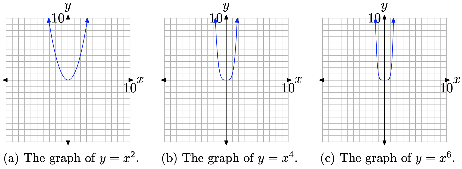
Figure $\PageIndex{1}$. Examples of the graph of $y=x^{n}$, when n is an even integer.

The graphs in Figure $\PageIndex{1}$ share an important trait. As you sweep your eyes from left to right, each graph falls from positive infinity, wiggles through the origin, then rises back to positive infinity.

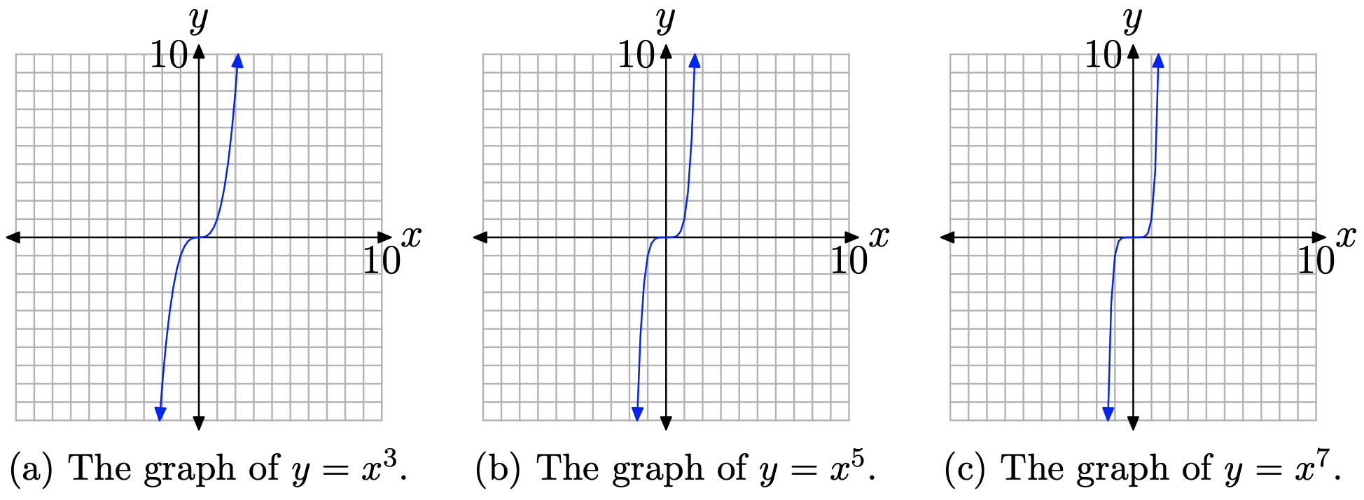
Next, let’s examine the graph of $y=x^{n}$, when n is odd. Again, a table of points or a graphing calculator will help produce the graphs of $y=x^{3}, y=x^{5},$ and $y=x^{7}$, as shown in Figure $\PageIndex{2}$(a), (b), and (c), respectively.

The graphs in Figure $\PageIndex{2}$ share an important trait. As you sweep your eyes from left to right, each graph rises from negative infinity, wiggles through the origin, then rises up to positive infinity.

The behavior shown in Figure $\PageIndex{1}$ and Figure $\PageIndex{2}$ is typical.

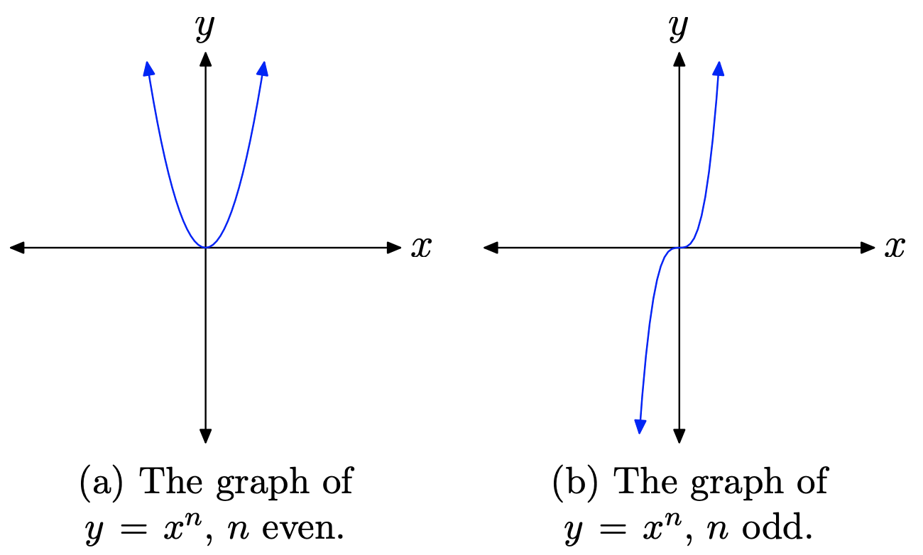
Figure $\PageIndex{2}$. Examples of the graph of $y=x^{n}$, when n is an odd integer.

Property 9

When n is an even natural number, the graph of $y=x^{n}$ will look like that shown in Figure $\PageIndex{3}$(a). If n is an odd natural number, then the graph of $y=x^{n}$ will be similar to that shown in Figure $\PageIndex{3}$(b).

When n is even, as you sweep your eyes from left to right, the graph of $y=x^{n}$ falls from positive infinity, wiggles through the origin, then rises back to positive infinity.
If n is odd, as you sweep your eyes from left to right, the graph of $y=x^{n}$ rises from negative infinity, wiggles through the origin, then rises to positive infinity.

The Graph of $y=a x^{n}$

Now that we know the general shape of the graph of $y=x^{n}$, let’s scale this function by multiplying by a constant, as in $y=a x^{n}$.

In our study of the parabola, we learned that if we multiply by a factor of a, where a > 1, then we will stretch the graph in the vertical direction by a factor of a. Conversely, if we multiply the graph by a factor of a, where 0 < a < 1, then we will compress the graph in the vertical direction by a factor of 1/a. If a < 0, then not only will we scale the graph, but multiplying by this factor will also reflect the graph across the horizontal axis.

Let’s look at a few examples.

Example $\PageIndex{4}$

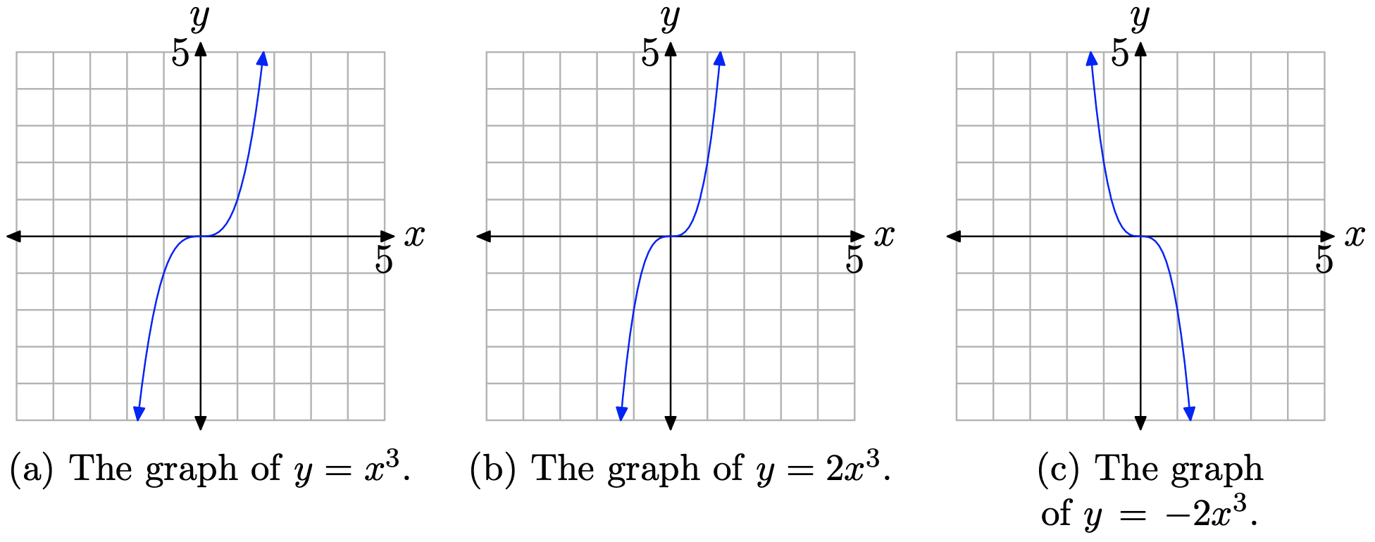
Sketch the graph of $y=-2 x^{3}$.

Solution

We know what the graph of $y=x^{3}$ looks like. As we sweep our eyes from left to right, the graph rises from negative infinity, wiggles through the origin, then rises to positive infinity. This behavior is shown in Figure $\PageIndex{4}$(a).

If we multiply by a factor of 2, then we stretch the original graph by a factor of 2 in the vertical direction. The graph of $y=2 x^{3}$ is shown in Figure $\PageIndex{4}$(b). Note the stretching in the vertical direction.

Finally, if we negate by multiplying by −2, this will stretch the graph by a factor of 2, as in Figure $\PageIndex{4}$(b), but it will also reflect the graph across the x-axis. The graph of $y=-2 x^{3}$ is shown in Figure $\PageIndex{4}$(c).

Figure $\PageIndex{4}$. Scaling by −2 stretches vertically by a factor of 2, then reflects the graph across the x-axis.

Let’s look at another example.

Example $\PageIndex{5}$

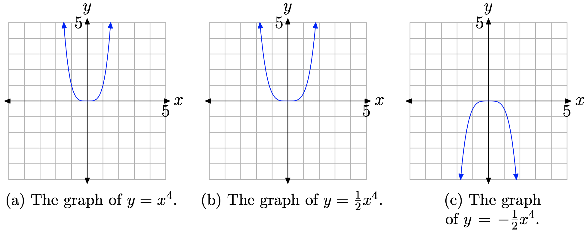
Sketch the graph of $y=-\frac{1}{2} x^{4}$

Solution

We know what the graph of $y=x^{4}$ looks like. As we sweep our eyes from left to right, the graph falls from positive infinity, wiggles through the origin, then rises back to positive infinity. This behavior is shown in Figure $\PageIndex{5}$(a).

If we multiply by 1/2, then we will compress the graph by a factor of 2. Note that the graph of $y=\frac{1}{2} x^{4}$ in Figure $\PageIndex{5}$(b) is compressed by a factor of 2 in the vertical direction.

Finally, if we multiply by −1/2, not only will we compress the graph by a factor of 2, we will also reflect the graph across the x-axis. The graph of $y=-\frac{1}{2} x^{4}$ is shown in Figure $\PageIndex{5}$(c).

Figure $\PageIndex{5}$. Scaling by −1/2 compresses vertically by a factor of 2, then reflects the graph across the x-axis.

Hopefully, at this point you can now sketch the graph of $y=a x^{n}$ for any real number a and any natural number n, either even or odd, without the use of a calculator. Let’s put this new-found knowledge to use in investigating the end-behavior of polynomials.

End Behavior

Consider the polynomial $p(x)=x^{3}-7 x^{2}+7 x+15$.

Here’s a key fact that we will use to determine the end-behavior of any polynomial.

Property 13

A polynomial’s end-behavior is completely determined by its leading term. That is, the end-behavior of the graph of the polynomial will match the end-behavior of the graph of its leading term.

In a moment, we will show why this property is true. In the meantime, let’s accept the veracity of this statement and apply it to the polynomial defined by equation (12). The leading term of the polynomial $p(x)=x^{3}-7 x^{2}+7 x+15$ is $x^{3}$. We know the end behavior of graph of $y=x^{3}$. As we sweep our eyes from left to right, the graph of $y=x^{3}$ will rise from negative infinity, wiggle through the origin, then continue to rise to positive infinity. We pictured this behavior earlier in Figure $\PageIndex{4}$(a).

Property 13 tells us that the graph of the polynomial $p(x)=x^{3}-7 x^{2}+7 x+15$ will exhibit the same end-behavior as the graph of its leading term, $y=x^{3}$. We can predict that, as we sweep our eyes from left to right, the graph of the polynomial $p(x)=x^{3}-7 x^{2}+7 x+15$ will rise from negative infinity, wiggle a bit, then rise to positive infinity. We don’t know what happens in-between, but we do know what happens at far left- and right-hand ends.

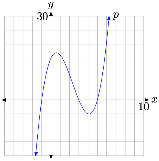
Our conjecture is verified by drawing the graph (use a graphing calculator). The graph of the polynomial $p(x)=x^{3}-7 x^{2}+7 x+15$ is shown in Figure $\PageIndex{6}$. Sure enough, as we sweep our eyes from left to right, the graph in Figure $\PageIndex{6}$ rises from negative infinity as predicted, wiggles a bit, then continues its rise to positive infinity.

Figure $\PageIndex{6}$. Note that this graph of $p(x)=x^{3}-7 x^{2}+7 x+15$ has the same end-behavior as the graph of $y=x^{3}$.

Why Does it Work? Why does Property 13 predict so accurately the end-behavior of this polynomial?

\[p(x)=x^{3}-7 x^{2}+7 x+15 \nonumber \]

We can demonstrate why by first factoring out the leading term.

\[p(x)=x^{3}\left(1-\frac{7}{x}+\frac{7}{x^{2}}+\frac{15}{x^{3}}\right) \nonumber \]

Now, ask the following question. What happens to the polynomial as we move to the right end? That is, what happens to the polynomial as we use large values of x, such as 1 000, 10 000, or even 100 000?

Consider the fraction $\dfrac{7}{x}$. Because the numerator is fixed at 7, and the denominator is getting bigger and bigger (growing without bound), the fraction is getting closer and closer to zero. Calculus students would use the notation

\[\lim _{x \rightarrow \infty} \frac{7}{x}=0 \nonumber \]

Don’t be put off by the notation. We’re using sophisticated mathematical notation for a very simple idea that says “As x approaches infinity, the fraction 7/x approaches zero.”

Using similar reasoning, each of the fractions in equation (14) go to zero as x goes to infinity (increases without bound). Thus, as x gets larger and larger (as we move further and further to the right),

\[\lim _{x \rightarrow \infty} p(x)=\lim _{x \rightarrow \infty} x^{3}\left(1-\frac{7}{x}+\frac{7}{x^{2}}+\frac{15}{x^{3}}\right) \approx x^{3}(1-0+0+0+0) \approx x^{3} \nonumber \]

That is, as x increases without bound, the graph of $p(x)=x^{3}-7 x^{2}+7 x+15$ should approximate the graph of $y=x^{3}$.

Using similar reasoning, each of the fractions in equation (14) go to zero as x goes to minus infinity. That is, if you are putting in numbers for x such as −1 000, −10 000, −100 000, and the like, the fractions in equation (14) will go to zero. Hence, the polynomial p(x) must still approach its leading term x 3 for very small values of x (as x approaches $-\infty$).

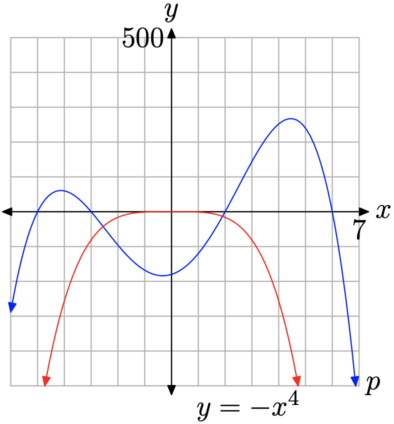
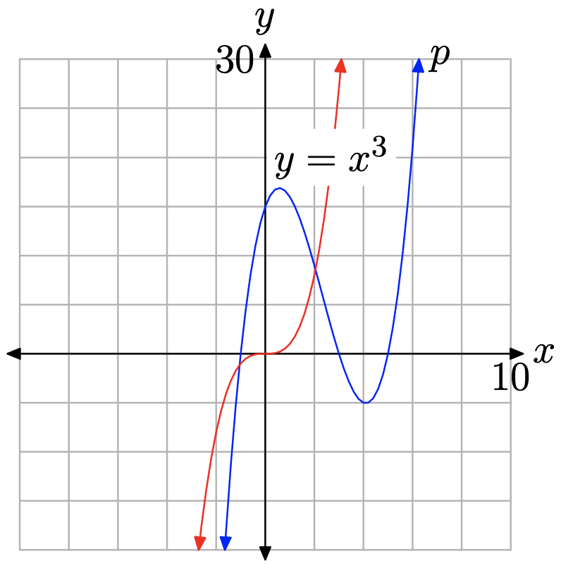
If you superimpose the graph of $y=x^{3}$ on the graph of $p(x)=x^{3}-7 x^{2}+7 x+15$, as in Figure $\PageIndex{7}$, it’s clear that the polynomial p has the same end-behavior as the graph of its leading term $y=x^{3}$.

Figure $\PageIndex{7}$. As you move to the extreme left or right, the graph of $p(x)=x^{3}-7 x^{2}+7 x+15$ approaches the graph of its leading term $y=x^{3}$.

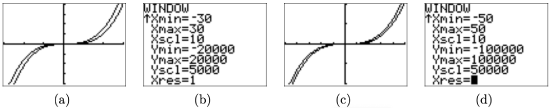
You can provide a more striking demonstration of the validity of the claim in equation (15) by plotting both the polynomial p and its leading term $y=x^{3}$ on your calculator, then zooming out by adjusting the window parameters as shown in Figure $\PageIndex{8}$(b). Note how the graph of $p(x)=x^{3}-7 x^{2}+7 x+15$ more closely resembles the graph of its leading term $y=x^{3}$, at least at the right and left edges of the viewing window. When we zoom further out, by adjusting the window parameters as shown in Figure $\PageIndex{8}$(d), note how that graph of p approaches the graph of its leading term $y=x^{3}$ even more closely at each edge of the viewing window.

Figure $\PageIndex{8}$. Zooming out clearly demonstrates that the end-behavior of $p(x)=x^{3}-7 x^{2}+7 x+15$ matches that of its leading term $y=x^{3}$.

Let’s look at another example.

Example $\PageIndex{6}$

Consider the polynomial $p(x)=-x^{4}+37 x^{2}+24 x-180$. Comment on the end-behavior of p and use your graphing calculator to sketch its graph.

Solution

The leading term of $p(x)=-x^{4}+37 x^{2}+24 x-180$ is $y=-x^{4}$. We know the end-behavior of the graph of the leading term. As we sweep our eyes from left to right, the graph of $y=-x^{4}$ rises from negative infinity, wiggles through the origin, then falls back to minus infinity. The graph of p should exhibit the same end-behavior. Indeed, in Figure $\PageIndex{9}$, note that the graph of $y=-x^{4}$ and $y=-x^{4}+37 x^{2}+24 x-180$ both share the same end-behavior.

Figure $\PageIndex{9}$. The polynomial $p(x)=-x^{4}+37 x^{2}+24 x-180$ has the same end-behavior as the graph of its leading term $y=-x^{4}$.

The Graph of \(y=x^{n}\)

The Graph of \(y=a x^{n}\)

End Behavior