3.3: Real Zeros of Polynomials

Math 370 Learning Objectives

• Rational Roots of Polynomials: Use the Rational Roots Theorem to help determine the rational zeros of a given polynomial.
• Finding Zeros of Polynomials Using Theory: Solve polynomial equations and inequalities with the help of the Rational Roots Theorem.
• Finding Zeros of Polynomials Using Technology: Use technology to assist in approximating zeros of a polynomial.

In Section 3.2, we found that we can use synthetic division to determine if a given real number is a zero of a polynomial function. This section presents results which will help us determine good candidates to test using synthetic division. There are two approaches to the topic of finding the real zeros of a polynomial. The first approach (which is gaining popularity) is to use a little bit of Mathematics followed by a good use of graphing technology. The second approach (for purists) makes good use of mathematical machinery (theorems) only. For completeness, we include the two approaches but in separate subsections.

---

Bounding Zeros of Polynomials

Before we look at the two main approaches to finding the zeros of polynomial functions, we present two theorems, the first of which is due to the famous mathematician Augustin Cauchy. It gives us an interval on which all of the real zeros of a polynomial can be found.

Theorem \(\PageIndex{1}\): Cauchy's Bounding Theorem

Suppose \[f(x)=a_{n} x^{n}+a_{n-1} x^{n-1}+\ldots+a_{1} x+a_{0} \nonumber \]is a polynomial of degree \(n\) with \(n \geq 1\). Let \(M\) be the largest of the numbers: \(\dfrac{\left|a_{0}\right|}{\left|a_{n}\right|}, \dfrac{\left|a_{1}\right|}{\left|a_{n}\right|}, \ldots, \dfrac{\left|a_{n-1}\right|}{\left|a_{n}\right|}\). Then all the real zeros of \(f\) lie in in the interval \([-(M+1), M+1]\).

The proof of this fact is not easily explained within the confines of this text. Like many of the results in this section, Cauchy’s Bound is best understood with an example.

Example \( \PageIndex{1} \)

Let \(f(x)=2 x^{4}+4 x^{3}-x^{2}-6 x-3\). Determine an interval which contains all of the real zeros of \(f\).

Solution

To find the \(M\) stated in Cauchy’s Bound, we take the absolute value of the leading coefficient, in this case \(|2|=2\) and divide it into the largest (in absolute value) of the remaining coefficients, in this case \(|-6|=6\). This yields \(M = 3\) so it is guaranteed that all of the real zeros of \(f\) lie in the interval \([−4, 4]\).

---

Rational Roots of Polynomials

Whereas the previous result tells us where we can find the real zeros of a polynomial, the next theorem gives us a list of possible real zeros.

Theorem \(\PageIndex{2}\): Rational Zeros Theorem¹

Suppose \[f(x)=a_{n} x^{n}+a_{n-1} x^{n-1}+\ldots+a_{1} x+a_{0}\nonumber \]is a polynomial of degree \(n\) with \(n \geq 1\), and \(a_{0}, a_{1}, \ldots a_{n}\) are integers. If \(r\) is a rational zero of \(f\), then \(r\) is of the form \(\pm \dfrac{p}{q}\), where \(p\) is a factor of the constant term \(a_{0}\), and \(q\) is a factor of the leading coefficient \(a_{n}\).

Proof

Suppose \(c\) is a zero of \(f\) and \(c=\dfrac{p}{q}\) in lowest terms. This means \(p\) and \(q\) have no common factors. Since \(f(c) = 0\), we have

\(a_{n}\left(\dfrac{p}{q}\right)^{n}+a_{n-1}\left(\dfrac{p}{q}\right)^{n-1}+\ldots+a_{1}\left(\dfrac{p}{q}\right)+a_{0}=0\).

Multiplying both sides of this equation by \(q^{n}\), we clear the denominators to get

\(a_{n} p^{n}+a_{n-1} p^{n-1} q+\ldots+a_{1} p q^{n-1}+a_{0} q^{n}=0\)

Rearranging this equation, we get

\(a_{n} p^{n}=-a_{n-1} p^{n-1} q-\ldots-a_{1} p q^{n-1}-a_{0} q^{n}\)

Now, the left hand side is an integer multiple of \(p\), and the right hand side is an integer multiple of \(q\). (Can you see why?) This means \(a_{n} p^{n}\) is both a multiple of \(p\) and a multiple of \(q\). Since \(p\) and \(q\) have no common factors, \(a_{n}\) must be a multiple of \(q\). If we rearrange the equation

\(a_{n} p^{n}+a_{n-1} p^{n-1} q+\ldots+a_{1} p q^{n-1}+a_{0} q^{n}=0\)

as

\(a_{0} q^{n}=-a_{n} p^{n}-a_{n-1} p^{n-1} q-\ldots-a_{1} p q^{n-1}\)

we can play the same game and conclude \(a_{0}\) is a multiple of \(p\), and we have the result.

The Rational Zeros Theorem gives us a list of numbers to try in our synthetic division and that is a lot nicer than simply guessing. If none of the numbers in the list are zeros, then either the polynomial has no real zeros at all, or all of the real zeros are irrational numbers.

Example \( \PageIndex{2} \)

Let \(f(x)=2 x^{4}+4 x^{3}-x^{2}-6 x-3\). Use the Rational Zeros Theorem to list all of the possible rational zeros of \(f\).

Solution

To generate a complete list of rational zeros, we need to take each of the factors of constant term, \(a_{0}=-3\), and divide them by each of the factors of the leading coefficient \(a_{4}=2\). The factors of \(−3\) are \(\pm 1\) and \(\pm 3\). Since the Rational Zeros Theorem tacks on a \(\pm\) anyway, for the moment, we consider only the positive factors \(1\) and \(3\). The factors of \(2\) are \(1\) and \(2\), so the Rational Zeros Theorem gives the list \(\left\{\pm \dfrac{1}{1}, \pm \dfrac{1}{2}, \pm \dfrac{3}{1}, \pm \dfrac{3}{2}\right\}\) or \(\left\{\pm \dfrac{1}{2}, \pm 1, \pm \dfrac{3}{2}, \pm 3\right\}\).

Subsection Footnotes

¹ The Rational Zeros Theorem is also commonly referred to as the Rational Roots Theorem.

---

Finding Zeros of Polynomials Using Theory

The Rational Zeros Theorem allows us enough mathematical ability to solve polynomial equations and inequalities that were impossible for us to solve in the past.

Example \( \PageIndex{3} \)

1. Find all of the real solutions to the equation \(2 x^{5}+6 x^{3}+3=3 x^{4}+8 x^{2}\).
2. Solve the inequality \(2 x^{5}+6 x^{3}+3 \leq 3 x^{4}+8 x^{2}\).
3. Interpret your answer to part 2 graphically, and verify using graphing technology.

Solution

1. Finding the real solutions to \[2 x^{5}+6 x^{3}+3=3 x^{4}+8 x^{2}\nonumber \]is the same as finding the real solutions to \[2 x^{5}-3 x^{4}+6 x^{3}-8 x^{2}+3=0.\nonumber \]In other words, we are looking for the real zeros of \[p(x)=2 x^{5}-3 x^{4}+6 x^{3}-8 x^{2}+3.\nonumber\]By Cauchy's Bound, we know the real zeros of this polynomial must exist in the interval \( \left[ -4, 4 \right] \). The Rational Zeros Theorem gives us the candidate zeros \( \left\{ \pm\frac{1}{1}, \pm \frac{2}{1}, \pm \frac{4}{1}, \pm \frac{8}{1}, \pm \frac{1}{2} \right\} \). Using the techniques developed in this chapter, we get \[\begin{array}{rrrrr} 1\mid&2&-3&6&-8&0&3\\ &\downarrow&2&-1&5&-3&-3\\ \hline 1\mid&2&-1&5&-3&-3&\boxed{0}\\ &\downarrow&2&1&6&3\\ \hline -\dfrac{1}{2}\mid&2&1&6&3&\boxed{0}\\ &\downarrow&-1&0&-3\\ \hline &2&0&6&\boxed{0} \end{array}\nonumber \]The quotient polynomial is \(2 x^{2}+6\) which has no real zeros so we get \(x=-\dfrac{1}{2}\) and \(x = 1\).
2. To solve this nonlinear inequality, we follow the same guidelines set forth in Section 2.4: we get \(0\) on one side of the inequality and construct a sign diagram. Our original inequality can be rewritten as \[2 x^{5}-3 x^{4}+6 x^{3}-8 x^{2}+3 \leq 0.\nonumber \]We found the zeros of \(p(x)=2 x^{5}-3 x^{4}+6 x^{3}-8 x^{2}+3\) in part 1 to be \(x=-\dfrac{1}{2}\) and \(x = 1\). We construct our sign diagram as before.

   
   Figure \( \PageIndex{1} \)

   The solution to \(p(x)<0\) is \(\left(-\infty,-\dfrac{1}{2}\right)\), and we know \(p(x) = 0\) a \(x=-\dfrac{1}{2}\) and \(x = 1\). Hence the solution to \(p(x) \leq 0\) is \(\left(-\infty,-\dfrac{1}{2}\right] \cup\{1\}\).
3. To interpret this solution graphically, we set \(f(x)=2 x^{5}+6 x^{3}+3\) and \(g(x)=3 x^{4}+8 x^{2}\). We recall that the solution to \(f(x) \leq g(x)\) ) is the set of \(x\) values for which the graph of \(f\) is below the graph of \(g\) (where \(f(x)<g(x)\)) ) along with the \(x\) values where the two graphs intersect \((f(x) = g(x)\). Graphing \(f\) (in blue) and \(g\) (in black) using Desmos produces Figure \( \PageIndex{2}A \). (The end behavior should tell you which is which.) We see that the graph of \(f\) is below the graph of \(g\) on \(\left(-\infty,-\dfrac{1}{2}\right)\). However, it is difficult to see what is happening near \(x = 1\). Zooming in, we see that the graphs of \(f\) and \(g\) do intersect at \(x = 1\), but the graph of \(g\) remains below the graph of \(f\) on either side of \(x =1\).

     
   Figures \( \PageIndex{2}A \) (left) and \( \PageIndex{2}B \) (right)

Our last example revisits an application from the Exercises in Section 3.1.

Example \( \PageIndex{4} \)

Suppose the profit \(P\), in thousands of dollars, from producing and selling \(x\) hundred LCD TVs is given by \(P(x)=-5 x^{3}+35 x^{2}-45 x-25,\) where \(0 \leq x \leq 10.07\). How many TVs should be produced to make a profit? Check your answer using a graphing technology.

Solution

To "make a profit" means to solve \(P(x)=-5 x^{3}+35 x^{2}-45 x-25>0\), which we do analytically using a sign diagram. To simplify things, we first factor out the \(−5\) common to all the coefficients to get \(-5\left(x^{3}-7 x^{2}+9 x-5\right)>0\), so we can just focus on finding the zero of \(f(x)=x^{3}-7 x^{2}+9 x+5\).

The possible rational zeros of \(f\) are \(\pm 1\) and \(\pm 5\), and going through the usual computations, we find \(x=5\) is the only rational zero. Using this, we factor \[f(x)=x^{3}-7 x^{2}+9 x+5=(x-5)\left(x^{2}-2 x-1\right),\nonumber \]and we find the remaining zeros by applying the Quadratic Formula to \(x^{2}-2 x-1=0\). We find three real zeros, \(x=1-\sqrt{2}=-0.414 \ldots\), \(x=1+\sqrt{2}=2.414 \ldots\), and \(x=5\), of which only the last two fall in the applied domain of \([0, 10.07]\). We choose \(x = 0\), \(x = 3\) and \(x = 10.07\) as our test values and plug them into the function \(P(x)=-5 x^{3}+35 x^{2}-45 x-25 \left(\text { not } f(x)=x^{3}-7 x^{2}+9 x-5\right)\) to get the sign diagram in Figure \( \PageIndex{3} \).

Figure \( \PageIndex{3} \)

We see immediately that \(P(x)>0\) on \((1+\sqrt{2}, 5)\). Since \(x\) measures the number of TVs in hundreds, \(x=1+\sqrt{2}\) corresponds to \(241.4\) TVs. Since we can’t produce a fractional part of a TV, we need to choose between producing \(241\) and \(242\) TVs. From Figure \( \PageIndex{3} \), we see that \(P(2.41)<0\) but \(P(2.42)>0\) so, in this case we take the next larger integer value and set the minimum production to \(242\) TVs. At the other end of the interval, we have \(x = 5\) which corresponds to \(500\) TVs. Here, we take the next smaller integer value, \(499\) TVs to ensure that we make a profit. Hence, in order to make a profit, at least \(242\), but no more than \(499\) TVs need to be produced. To check our answer using Desmos, we graph \(y = P(x)\). Figure \( \PageIndex{4} \) shows that Desmos' approximations bear out our analysis.

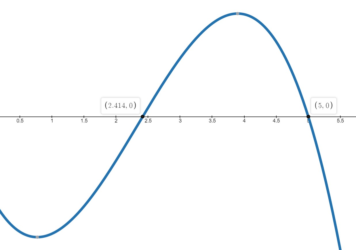
Figure \( \PageIndex{4} \)

---

Finding Zeros of Polynomials Using Technology

At this stage, we know not only the interval in which all of the zeros of \(f(x)=2 x^{4}+4 x^{3}-x^{2}-6 x-3\) are located, but we also know some potential candidates. We can now use technology to help us determine all of the real zeros of \(f\), as illustrated in the next example.

Example \( \PageIndex{5} \)

Let \(f(x)=2 x^{4}+4 x^{3}-x^{2}-6 x-3\).

1. Graph \(y = f(x)\) using graphing technology and the interval obtained in Example \( \PageIndex{1} \) as a guide.
2. Use the graph to shorten the list of possible rational zeros obtained in Example \( \PageIndex{2} \).
3. Use synthetic division to find the real zeros of \(f\), and state their multiplicities.

Solution

1. In Example \( \PageIndex{1} \), we determined all of the real zeros of \(f\) lie in the interval \([−4, 4]\). We set our window accordingly and get Figure \( \PageIndex{5} \).

   
   Figure \( \PageIndex{5} \)

2. In Example \( \PageIndex{2} \), we learned that any rational zero of \(f\) must be in the list \(\left\{\pm \dfrac{1}{2}, \pm 1, \pm \dfrac{3}{2}, \pm 3\right\}\). From the graph, it looks as if we can rule out any of the positive rational zeros, since the graph seems to cross the \(x\)-axis at a value just a little greater than \(1\). On the negative side, \(−1\) looks good, so we try that for our synthetic division. \[ \begin{array}{rrrrrr} -1\mid & 2 & 4 & -1 & -6 & -3 \\ &\downarrow & -2 & -2 & 3 & 3 \\ \hline &2 & 2 & -3 & -3 & \boxed{0} \end{array}\nonumber \]We have a winner! Remembering that \(f\) was a fourth-degree polynomial, we know that our quotient is a third-degree polynomial. If we can do one more successful division, we will have knocked the quotient down to a quadratic, and, if all else fails, we can use the Quadratic Formula to find the last two zeros. Since there seems to be no other rational zeros to try, we continue with \(−1\). Also, the shape of the crossing at \(x = −1\) leads us to wonder if the zero \(x = −1\) has multiplicity \(3\). \[ \begin{array}{rrrrrr} -1\mid & 2 & 4 & -1 & -6 & -3 \\ &\downarrow & -2 & -2 & 3 & 3 \\ \hline -1\mid&2 & 2 & -3 & -3 & \boxed{0}\\ &\downarrow & -2 & 0 & 3 \\ \hline &2 & 0 & -3 & \boxed{0}\end{array}\nonumber \]Success! Our quotient polynomial is now \(2 x^{2}-3\). Setting this to zero gives \(2 x^{2}-3=0\), or \(x^{2}=\dfrac{3}{2}\), which gives us \(x=\pm \dfrac{\sqrt{6}}{2}\). Concerning multiplicities, based on our division, we have that \(−1\) has a multiplicity of at least \(2\). The Factor Theorem tells us our remaining zeros, \(\pm \dfrac{\sqrt{6}}{2}\), each have multiplicity at least \(1\). However, Theorem 3.2.4 tells us \(f\) can have at most \(4\) real zeros, counting multiplicity, and so we conclude that \(−1\) is of multiplicity exactly \(2\) and \(\pm \dfrac{\sqrt{6}}{2}\) each has multiplicity \(1\).

It is interesting to note that we could greatly improve on the graph of \(y = f(x)\) in the previous example given to us by Desmos. For instance, from our determination of the zeros of \(f\) and their multiplicities, we know the graph crosses at \(x=-\dfrac{\sqrt{6}}{2} \approx-1.22\) then turns back upwards to touch the \(x\)−axis at \(x = −1\). This tells us that, despite what the calculator showed us the first time, there is a relative maximum occurring at \(x = −1\) and not a "flattened crossing" as we originally believed.² After resizing the window (see Figure \( \PageIndex{6} \)), we see not only the relative maximum but also a relative minimum just to the left of \(x = −1\) which shows us, once again, that Mathematics enhances the technology, instead of vice-versa.

Figure \( \PageIndex{6} \)

Our next example shows how even a mild-mannered polynomial can cause problems.

Example \( \PageIndex{6} \)

Let \(f(x)=x^{4}+x^{2}-12\).

1. Use Cauchy’s Bound to determine an interval in which all of the real zeros of \(f\) lie.
2. Use the Rational Zeros Theorem to determine a list of possible rational zeros of \(f\).
3. Graph \(y = f(x)\) using graphing technology.
4. Find all of the real zeros of \(f\) and their multiplicities.

Solution

1. Applying Cauchy’s Bound, we find \(M = 12\), so all of the real zeros lie in the interval \([−13, 13]\).
2. Applying the Rational Zeros Theorem with constant term \(a_{0}=-12\) and leading coefficient \(a_{4}=1\), we get the list \(\{\pm 1, \pm 2, \pm 3, \pm 4, \pm 6, \pm 12\}\).
3. Graphing \(y = f(x)\) on the interval \([−13, 13]\) produces Figure \( \PageIndex{7}A \). Zooming in a bit gives Figure \( \PageIndex{7}B \). Based on the graph, none of our rational zeros will work. (Do you see why not?)

     
   Figures \( \PageIndex{7}A \) (left) and \( \PageIndex{7}B \) (right)

4. From the graph, we know \(f\) has two real zeros, one positive, and one negative. Our only hope at this point is to try and find the zeros of \(f\) by setting \(f(x)=x^{4}+x^{2}-12=0\) and solving.
   If we stare at this equation long enough, we may recognize it as a "quadratic in disguise" or "quadratic in form." In other words, we have three terms: \(x^{4}\), \(x^{2}\) and \(12\), and the exponent on the first term, \(x^{4}\), is exactly twice that of the second term, \(x^{2}\). We may rewrite this as \[\left(x^{2}\right)^{2}+\left(x^{2}\right)-12=0.\nonumber \]To better see the forest for the trees, we momentarily replace \(x^{2}\) with the variable \(u\). In terms of \(u\), our equation becomes \(u^{2}+u-12=0\), which we can readily factor as \((u + 4)(u − 3) = 0\). In terms of \(x\), this means \(x^{4}+x^{2}-12=\left(x^{2}-3\right)\left(x^{2}+4\right)=0\). We get \(x^{2}=3\), which give us \(x=\pm \sqrt{3}\), or \(x^{2}=-4\), which admits no real solutions. Since, \(\sqrt{3} \approx 1.73\), the two zeros match what we expected from the graph.
   In terms of multiplicity, the Factor Theorem guarantees \((x-\sqrt{3})\) and \((x+\sqrt{3})\) are factors of \(f(x)\). Since \(f(x)\) can can be factored as \[f(x)=\left(x^{2}-3\right)\left(x^{2}+4\right),\nonumber \]and \(x^{2}+4\) has no real zeros, the quantities \((x-\sqrt{3})\) and \((x+\sqrt{3})\) must both be factors of \(x^{2}-3\). According to Theorem 3.2.4, \(x^{2}-3\) can have at most 2 zeros, counting multiplicity, hence each of \(\pm \sqrt{3}\) is a zero of \(f\) of multiplicity \(1\).

The technique used to factor \(f(x)\) in Example \( \PageIndex{6} \) is called \(u\)-substitution. We shall see more of this technique in Section 5.2. In general, substitution can help us identify a "quadratic in disguise" provided that there are exactly three terms and the exponent of the first term is exactly twice that of the second. It is entirely possible that a polynomial has no real roots at all, or worse, it has real roots but none of the techniques discussed in this section can help us find them exactly. In the latter case, we are forced to approximate, which in this subsection means using Desmos to find the intersection points of \( f(x) \) and the \( x \)-axis.

Subsection Footnotes

² This is an example of what is called "hidden behavior."