2.4: Introduction to Proofs in Trigonometry

Suggested Prerequisite Topics

This section is designed assuming you understand the following topics from Algebra.

• Simplify sums, differences, products, and quotients of algebraic expressions
• Evaluate functions at algebraic arguments
• Understand and use the piecewise definition of the absolute value function
• Use technology to graph functions

Learning Objectives

• Simplify a trigonometric expression.
• Rewrite a trigonometric expression in terms of sines and cosines.
• Simplify an algebraic expression by performing a trigonometric substitution.
• Determine the plausibility of an identity graphically and understand this does not prove an identity (but can disprove an identity).
• Prove basic trigonometric identities.

We have already been introduced to several fundamental identities in Trigonometry. Namely, the Ratio, Reciprocal, and Pythagorean Identities. We then spent most of that section using those identities to help us evaluate trigonometric functions. In this section, we learn how to use those identities to simplify expressions involving trigonometric functions. We then start dipping our toes into proving identities.

Simplifying Expressions Involving Trigonometric Functions

Recall that an expression (or mathematical expression) is a combination of symbols that are mathematically "well-formed." The mathematical symbols can include numbers (constants), variables, operations (e.g., addition, subtraction, multiplication, etc.), functions, brackets, and other grouping symbols to help determine the order of operations. The one symbol that is always missing from an expression is the equals sign (\( = \)).

Reminder: Equations versus Expressions

Equations have equals signs - expressions do not.

You solve equations, but you simplify expressions.

When we simplify an algebraic expression, we obtain a new expression that has the same values as the old one, but is easier to work with. For example, we can apply the distributive law and combine like terms to simplify\[ \begin{array}{rcl}
2 x(x-6)+3(x+2) & = & 2 x^2-12 x+3 x+6 \\
& = & 2 x^2-9 x+6 \\
\end{array} \nonumber \]The new expression is equivalent to the old one, that is, the expressions have the same value when we evaluate them at any value of \(\x\). For instance, you can check that, at \(x=3\), the expressions \( 2x(x-6) + 3(x+2) \) and \( 2x^2 - 9x + 6 \) become\[ \begin{array}{rcccl}
2(3)(3-6)+3(3+2) & = & 6(-3)+3(5) & = & -3 \\
2(3)^2-9(3)+6 & = & 18-27+6 & = & -3 \\
\end{array} \nonumber \]To simplify an expression containing trigonometric functions, we treat each function as a single variable. Compare the two calculations below:\[ \begin{array}{ccccc}
8 x y & - & 6 x y & = & 2 x y \\
8 \cos \left(\theta\right) \sin \left(\theta\right) & - & 6 \cos \left(\theta\right) \sin \left(\theta\right) & = & 2 \cos \left(\theta\right) \sin \left(\theta\right) \\
\end{array} \nonumber \]Both calculations are examples of combining like terms. In the second calculation, we treat \(\cos \left(\theta\right)\) and \(\sin \left(\theta\right)\) as variables, just as we treat \(x\) and \(y\) in the first calculation.

In Trigonometry, we are often tasked with simplifying expressions involving trigonometric functions. In doing so, we will use many of our skills from Algebra (e.g., simplifying compound rational expressions, factoring, distributing, etc.) in combination with the identities we have recently discovered (along with those we will soon discover). One strategy for simplifying a trigonometric expression is to reduce the number of different trigonometric functions involved. The following example showcases this process using the Ratio Identities.

Example \( \PageIndex{ 1 } \)

1. Simplify: \(\cos \left(\theta\right) \tan \left(\theta\right)+\sin \left(\theta\right)\)
2. Multiply: \( \left( \cos\left( \theta \right) + \sin\left( \theta \right) \right)^2 \)
3. Add: \( \frac{\cos\left( \theta \right)}{\sin\left( \theta \right)} + \frac{\sin\left( \theta \right)}{\cos\left( \theta \right)} \)
4. Simplify: \(3 \tan \left(A\right)+4 \tan \left(A\right)-2 \cos \left(A\right)\)
5. Simplify: \(2-\sin \left(B\right)+2 \sin \left(B\right)\)

Solutions

1. We apply the Ratio Identities to replace \(\tan \left(\theta\right)\) by \(\frac{\sin \left(\theta\right)}{\cos \left(\theta\right)}\) and obtain\[\begin{array}{rcl}
   \cos \left(\theta\right) \tan \left(\theta\right)+\sin \left(\theta\right) & = & \cos \left(\theta\right)\left(\frac{\sin \left(\theta\right)}{\cos \left(\theta\right)}\right)+\sin \left(\theta\right) \\
   & = & \sin \left(\theta\right)+\sin \left(\theta\right) \\
   & = & 2 \sin \left(\theta\right) \\
   \end{array} \nonumber \]
2. The instruction to multiply implies we need to square the binomial and simplify.\[ \begin{array}{rclcr}
   \left( \cos\left( \theta \right) + \sin\left( \theta \right) \right)^2 & = & \cos^2\left( \theta \right) + 2 \cos\left( \theta \right) \sin\left( \theta \right) + \sin^2\left( \theta \right) & \quad & (\text{Squaring the binomial}) \\
   & = & \cos^2\left( \theta \right) + \sin^2\left( \theta \right) + 2 \cos\left( \theta \right) \sin\left( \theta \right) & \quad & (\text{Commutative Property of Addition}) \\
   & = & 1 + 2 \cos\left( \theta \right) \sin\left( \theta \right) & \quad & (\text{Pythagorean Identity}) \\
   \end{array} \nonumber \]
3. While we could use the Ratio Identities to make an equivalent expression, the result would be \( \cot\left( \theta \right) + \tan\left( \theta \right)\). At that point, we would be stuck. Instead, let's use the Mathematical Mantra and perform some arithmetic before trying our new Trigonometry skills. Specifically, let's get a common denominator and perform the subtraction.\[ \begin{array}{rclcr}
   \dfrac{\cos\left( \theta \right)}{\sin\left( \theta \right)} + \dfrac{\sin\left( \theta \right)}{\cos\left( \theta \right)} & = & \dfrac{\cos\left( \theta \right)}{\sin\left( \theta \right)} \cdot \dfrac{\cos\left( \theta \right)}{\cos\left( \theta \right)} + \dfrac{\sin\left( \theta \right)}{\cos\left( \theta \right)} \cdot \dfrac{\sin\left( \theta \right)}{\sin\left( \theta \right)} & \quad & (\text{Multiplying each fraction by an expression} \\
   & & & & \text{equivalent to 1 to get common denominators}) \\
   & = & \dfrac{\cos^2\left( \theta \right)}{\cos\left( \theta \right) \sin\left( \theta \right)} + \dfrac{\sin^2\left( \theta \right)}{\cos\left( \theta \right)\sin\left( \theta \right)} & & \\
   \\
   & = & \dfrac{\cos^2\left( \theta \right) + \sin^2\left( \theta \right)}{\cos\left( \theta \right) \sin\left( \theta \right)} & \quad & (\text{Adding fractions with like denominators}) \\
   \\
   & = & \dfrac{1}{\cos\left( \theta \right) \sin\left( \theta \right)} & \quad & (\text{Pythagorean Identity}) \\
   \end{array} \nonumber \]
4. Combine like terms.\[3 \tan \left(A\right)+4 \tan \left(A\right)-2 \cos \left(A\right)=7 \tan \left(A\right)-2 \cos \left(A\right)\nonumber \]Note that \(\tan \left(A\right)\) and \(\cos \left(A\right)\) are not like terms.
5. Combine like terms.\[2-\sin \left(B\right)+2 \sin \left(B\right)=2+\sin \left(B\right)\nonumber \]Note that \(-\sin \left(B\right)\) means \(-1 \cdot \sin \left(B\right)\).

It is often easier to know how a trigonometric expression (an expression involving trigonometric functions) will simplify once you try simplification techniques. In Example \( \PageIndex{ 1a } \), most students new to Trigonometry would likely never have looked at \(\cos \left(\theta\right) \tan \left(\theta\right)+\sin \left(\theta\right)\) and thought, "Hey, I bet that simplifies down to something nice... like \( 2 \sin\left( \theta \right) \)." Luckily, as you move forward in Trigonometry (and mathematics), you develop an intuition for when an expression can be simplified; however, cultivating this intuition takes time and experimentation.

Checkpoint \(\PageIndex{1}\)

Simplify each expression.

1. \( \left( 1 - \cos\left( \theta \right) \right)\left( 1 + \cos\left( \theta \right) \right) \)
2. \(2 \cos \left(t\right)-4 \cos \left(w\right) \sin \left(w\right)+3 \cos \left(t\right)-2 \cos \left(w\right)\)

Answers

1. \( \sin^2\left( \theta \right) \)
2. \(5 \cos \left(t\right)-4 \cos \left(w\right) \sin \left(w\right)-2 \cos \left(w\right)\)

Caution

In Checkpoint \( \PageIndex{ 1b } \), note that \(\cos \left(t\right)\) and \(\cos \left(w\right)\) are not like terms. (We can choose values for \(t\) and \(w\) so that \(\cos \left(t\right)\) and \(\cos \left(w\right)\) have different values.)

Rewriting Trigonometric Expressions

It is often necessary, especially in Calculus, to rewrite a trigonometric expression in terms of a single trigonometric function. To do so, we must use identities.

Example \( \PageIndex{ 2 } \)

1. Rewrite \(\sin \left(\theta\right) \cos ^2 \left(\theta\right)\) as an expression involving only sums or differences of powers of \(\sin \left(\theta\right)\).
2. Rewrite \( \cot\left( \theta \right) \) in terms of only \( \cos\left( \theta \right) \).

Solutions

1. Using one of the alternate forms of the Pythagorean Identity, we replace \(\cos ^2 \left(\theta\right)\) with \(1-\sin ^2 \left(\theta\right)\) to get\[\begin{array}{rclcr}
   \sin \left(\theta\right) \cos ^2 \left(\theta\right) & = & \sin \left(\theta\right)\left(1-\sin ^2 \left(\theta\right)\right) & \quad & (\text{Pythagorean Identity}) \\
   \\
   & = & \sin \left(\theta\right)-\sin ^3 \left(\theta\right) & \quad & (\text {Distributive Law}) \\
   \end{array} \nonumber \]
2.    \[ \begin{array}{rclcr}
   \cot\left( \theta \right) & = & \dfrac{\cos\left( \theta \right)}{\sin\left( \theta \right)} & \quad & (\text{Ratio Identities}) \\
   \\
   & = & \dfrac{\cos\left( \theta \right)}{\pm \sqrt{1 - \cos^2\left( \theta \right)}} & \quad & (\text{Pythagorean Identities (alternate form)}) \\
   \\
   & = & \pm\dfrac{\cos\left( \theta \right)}{\sqrt{1 - \cos^2\left( \theta \right)}} & \quad & \\
   \end{array} \nonumber \]

If we graph the original expression from Example \( \PageIndex{ 2a } \) as \( y_1=\sin\left( x\right) \cos ^2 \left(x\right)\) and our resulting equivalent expression as \( y_2=\sin\left( x \right)-\sin ^3\left( x \right) \), we see that they have the same graph, as shown in Figure \( \PageIndex{ 1 } \) below.¹

Figure \( \PageIndex{ 1 } \)

This should convince us that \(\sin \left(\theta\right) \cos ^2 \left(\theta\right)\) truly is equivalent to \( \sin\left( x \right)-\sin ^3\left( x \right) \).

The results of Example \( \PageIndex{ 2 } \) can be thought of as two new identities,\[\sin \left(\theta\right) \cos ^2 \left(\theta\right)=\sin \left(\theta\right)-\sin ^3 \left(\theta\right) \quad \text{and} \quad \cot\left( \theta \right) = \pm\dfrac{\cos\left( \theta \right)}{\sqrt{1 - \cos^2\left( \theta \right)}},\nonumber \]however, before you get too concerned with having to memorize these as two more identities, let's be clear:

Unless formally stated as a theorem, there is no need to memorize the hundreds of identities we will create, prove, or encounter in Trigonometry.

This means that the only identities you are responsible for memorizing (so far) are the Reciprocal, Ratio, and Pythagorean Identities.

Checkpoint \( \PageIndex{ 2 } \)

1. Rewrite \(\sin ^2 \left(\alpha\right) \cos ^2 \left(\alpha\right)\) as an expression involving only sums or differences of powers of \(\cos \left(\alpha\right)\).
2. Verify your identity by graphing.

Answers

\(\cos ^2 \left(\alpha\right)-\cos ^4 \left(\alpha\right)\)

The following example is extremely useful in Calculus II (Integral Calculus).

Example \(\PageIndex{3}\)

Simplify the expression\[ \dfrac{3}{\sqrt{x^2 - 4}} \nonumber \]as much as possible by substituting \( 2\sec\left( \theta \right) \) for \( x \).

Solution

\[ \begin{array}{rclcr}
\dfrac{3}{\sqrt{x^2 - 4}} & = & \dfrac{3}{\sqrt{\left( 2\sec\left( \theta \right) \right)^2 - 4}} & \quad & (\text{Substituting } 2\sec\left( \theta \right) \text{ for }x) \\
\\
& = & \dfrac{3}{\sqrt{4\sec^2\left( \theta \right) - 4}} & \quad & (\text{Squaring}) \\
\\
& = & \dfrac{3}{\sqrt{4\left(\sec^2\left( \theta \right) - 1\right)}} & \quad & (\text{Factoring}) \\
\\
& = & \dfrac{3}{2\sqrt{\sec^2\left( \theta \right) - 1}} & \quad & (\text{Taking the square root of }4) \\
\\
& = & \dfrac{3}{2\sqrt{\tan^2\left( \theta \right)}} & \quad & (\text{Using the modified Pythagorean Identity }\tan^2\left( \theta \right) = \sec^2\left( \theta \right) - 1) \\
\\
& = & \dfrac{3}{2\left|\tan\left( \theta \right)\right|} & \quad & (\text{See comments below}) \\
\end{array} \nonumber \]

Our solution to Example \( \PageIndex{ 3 } \) needs some clarification to ensure you understand what happened. Most of the work should be understandable; however, two steps might throw you off.

First, from the Pythagorean Identities, we used the fact that\[ 1 + \tan^2\left( \theta \right) = \sec^2\left( \theta \right); \nonumber \]however, we modified this identity slightly by subtracting 1 from both sides to get\[ \tan^2\left( \theta \right) = \sec^2\left( \theta \right) - 1. \nonumber \]The implication of that subtle modification cannot be overstated.

Being comfortable with the available identities and willing to manipulate them as needed will play a critical role in your success in Trigonometry.

The second item that needs our attention is the mathematical equivalence\[ \sqrt{\tan^2\left( \theta \right)} = \left| \tan\left( \theta \right)\right|. \nonumber \]A lot of students forget about the absolute values. Let's focus on what is happening here.

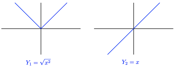
Suppose a friend of yours is claiming that the equation \(\sqrt{x^2}=x\) is an identity (this is the same as someone saying \( \sqrt{\tan^2\left( \theta \right)} = \tan\left( \theta \right) \)). As an astute mathematics student, you know that even though the equation is true for all positive values of \(x\), it is false for negative values of \(x\). For example, if \(x=-3\), then\[\sqrt{x^2}=\sqrt{(-3)^2}=\sqrt{9}=3\nonumber \]so \(\sqrt{x^2} \neq x\). The radical symbol \(\sqrt{ }\) stands for the principle square root - that is, the nonnegative square root. Therefore, the left side of the equation, \(\sqrt{x^2}\), is never negative. Thus, \(\sqrt{x^2}\) cannot equal \(x\) when \(x\) is a negative number. The equation is false for \(x<0\).

One way to see that \(\sqrt{x^2}\) and \(x\) are not equivalent is to compare the graphs of \(Y_1=\sqrt{x^2}\) and \(Y_2=x\), shown in Figure \( \PageIndex{ 2 } \) below. You can see that \(\sqrt{x^2}\) and \(x\) do not have the same value for \(x<0\).

Figure \( \PageIndex{ 2 } \)

Coming back to the last step in the solution of Example \( \PageIndex{ 3 } \), we should now feel comfortable saying that \( \sqrt{\tan^2\left( \theta \right)} \neq \tan\left( \theta \right) \) and we should be okay with saying\[ \sqrt{\tan^2\left( \theta \right)} = \left| \tan\left( \theta \right) \right|. \nonumber \]

Checking the Plausibility of Identities Graphically

Before jumping into how to rigorously prove a trigonometric identity, let's focus on ways to show that a claimed identity is not an identity.

From the discussion after Example \( \PageIndex{ 3 } \), we can see that, to check whether an equation might be an identity, we can compare graphs of \(Y_1\)=(left side of the equation) and \(Y_2=\) (right side of the equation). If the two graphs are identical, it is plausible that the equation is an identity. If the two graphs differ, the equation is not an identity.

Read that last paragraph again.

You cannot use a graph to prove an equation is an identity; however, you can use a graph to demonstrate it is not an identity.

This is crucial to understand. The following example provides some clarity.

Example \( \PageIndex{ 4 } \)

Which of the following equations might be identities?

1. \(\sin \left(2 \alpha\right)=2 \sin \left(\alpha\right)\)
2. \(\cos \left(x+\frac{\pi}{180}\right)=\cos \left(x\right)\)
3. \( \cos^2\left( \frac{\theta}{2} \right) = \frac{1 + \cos\left( \theta \right)}{2} \)

Solutions

1. Compare the graphs of \(y_1=\sin \left(2 x\right)\) and \(y_2=2 \sin \left(x\right)\). The Desmos graphs for both equations are shown in the figure below.

   

   Because there are two distinct graphs, the expressions \(\sin \left(2 x\right)\) and \(2 \sin \left(x\right)\) are not equivalent, and consequently, \(\sin \left(2 \alpha\right)=2 \sin \left(\alpha\right)\) is not an identity.
2. This time we graph \(y_1=\cos \left(x+\frac{\pi}{180}\right)\) and \(y_2=\cos \left(x\right)\).

   

   Although the graphs appear identical, when we zoom in, we see that the graphs are, indeed, not the same.

   

   The graphs are so close together that Desmos' resolution does not distinguish them, but zooming in reveals that they are not identical. Because the two graphs differ, the equation \(\cos \left(x+\frac{\pi}{180}\right)=\cos \left(x\right)\) is not an identity.
3. Letting \( y_1 = \cos^2\left( \frac{x}{2} \right) \) and \( y_2 = \frac{1 + \cos\left( x \right)}{2} \), we get the following graph from Desmos.

   

   These two graphs look identical; however, it is best to zoom in to double-check.

   

   No matter how much we zoom in, the two graphs appear identical. Therefore, we can say that it is plausible that \( \cos^2\left( \frac{\theta}{2} \right) = \frac{1 + \cos\left( \theta \right)}{2} \) is an identity.

Example \( \PageIndex{ 4 } \) has a few cautionary tales.

Caution: The Trouble with Technology

1. Example \( \PageIndex{ 4b } \) illustrates that graphs can be deceiving: even if two graphs look identical, it is always a good idea to zoom in or check some numerical values.
2. The related equation is not an identity if the two graphs are different.
3. Graphs cannot be used to prove that an equation is an identity.

Checkpoint \( \PageIndex{ 4 } \)

Use graphs to decide which of the following equations might be identities.

1. \(\cos \left(2 \theta\right)=2 \cos \left(\theta\right)\)
2. \(\cos \left(2 \theta\right)=\cos ^2 \left(\theta\right)-\sin ^2 \left(\theta\right)\)
3. \(\cos \left(\theta^2\right)=\cos ^2 \left(\theta\right)\)

Answers

(b)

Proving Identities

We have proved a trigonometric identity when we show that one trigonometric expression is equivalent to another. In Example \( \PageIndex{ 1a } \) we proved that the equation\[\cos \left(\theta\right) \tan \left(\theta\right)+\sin \left(\theta\right)=2 \sin \left(\theta\right)\nonumber \]is an identity; it is valid for all values of \(\theta\) (as long as the tangent function is defined).

A common strategy for proving an identity is to transform one side of the equation using equivalent expressions until it is identical to the other side. To help us choose the transformations at each step of the proof, we try to match the algebraic form of the final expression.

Example \( \PageIndex{ 5 } \)

Prove the identity\[1+\tan ^2 \left(t\right)=\dfrac{1}{\cos ^2 \left(t\right)}.\nonumber \]

Solution

By manipulating the left side of the equation, we will show that the expression \(1+\tan ^2 \left(t\right)\) is equivalent to \(\frac{1}{\cos ^2 \left(t\right)}\). First, we use the Ratio Identities to write the expression in terms of sines and cosines:\[1+\tan ^2 \left(t\right)=1+\left(\dfrac{\sin \left(t\right)}{\cos \left(t\right)}\right)^2=1+\dfrac{\sin ^2 \left(t\right)}{\cos ^2 \left(t\right)}\nonumber \]Next, we notice that the right side of the proposed identity has only one term, so we combine the terms on the left side. So that the fractions have the same denominator, we write 1 as \(\frac{\cos ^2 \left(t\right)}{\cos ^2 \left(t\right)}\).\[1+\dfrac{\sin ^2 \left(t\right)}{\cos ^2 \left(t\right)}=\dfrac{\cos ^2 \left(t\right)}{\cos ^2 \left(t\right)}+\dfrac{\sin ^2 \left(t\right)}{\cos ^2 \left(t\right)}=\dfrac{\cos ^2 \left(t\right)+\sin ^2 \left(t\right)}{\cos ^2 \left(t\right)}\nonumber \]Finally, we apply the Pythagorean Identity to the numerator.\[\dfrac{\cos ^2 \left(t\right)+\sin ^2 \left(t\right)}{\cos ^2 \left(t\right)}=\dfrac{1}{\cos ^2 \left(t\right)}\nonumber \]Thus, \(1+\tan ^2 \left(t\right)=\frac{1}{\cos ^2 \left(t\right)}\), and the identity is proved.

When you write out the proof of an identity, your goal is to transform the expression on one side of the identity into the expression on the other, showing one step of the calculation on each line of your proof. You can justify each step to the right of the calculation. The proof of the identity in the previous example would look like this:\[\begin{array}{rclcr}
\text{LHS} & = & 1+\tan ^2\left(t\right) & & \\
\\
& = & 1+\left(\dfrac{\sin \left(t\right)}{\cos \left(t\right)}\right)^2 & \quad & (\text {Ratio Identities}) \\
\\
& = & 1+\dfrac{\sin ^2 \left(t\right)}{\cos ^2 \left(t\right)} & \quad & (\text {Laws of Exponents}) \\
\\
& = & \dfrac{\cos ^2 \left(t\right)}{\cos ^2 \left(t\right)}+\dfrac{\sin ^2 \left(t\right)}{\cos ^2 \left(t\right)} & \quad & (\text {Get a common denominator to combine fractions}) \\
\\
& = & \dfrac{\cos ^2 \left(t\right)+\sin ^2 \left(t\right)}{\cos ^2 \left(t\right)} & \quad & (\text{Add fractions}) \\
\\
& = & \dfrac{1}{\cos ^2 \left(t\right)} & \quad & (\text {Pythagorean Identity}) \\
\\
& = & \text{RHS} & & \\
\end{array} \nonumber \]For now, we will focus on transforming the left side of an equation into the right side; however, as we move forward in Trigonometry, we will adopt the rule of thumb of transforming the more "complicated" side of the equation into the other side.

Exercise \(\PageIndex{6}\)

Prove the identity.\[ \left( \sin\left( \theta \right) - \cos\left( \theta \right) \right)^2 - 1 = -2 \sin\left( \theta \right) \cos\left( \theta \right) \nonumber \]

Solution

\[\begin{array}{rclcr}
\text{LHS} & = & \left( \sin\left( \theta \right) - \cos\left( \theta \right) \right)^2 - 1 & & \\
\\
& = & \sin^2\left( \theta \right) - 2 \cos\left( \theta \right) \sin\left( \theta \right) + \cos^2\left( \theta \right) - 1 & \quad & (\text {Squaring the binomial}) \\
\\
& = & \sin^2\left( \theta \right) + \cos^2\left( \theta \right) - 1 - 2 \cos\left( \theta \right) \sin\left( \theta \right) & \quad & (\text {Commutative Property of Addition}) \\
\\
& = & 1 - 1 - 2 \cos\left( \theta \right) \sin\left( \theta \right) & \quad & (\text {Pythagorean Identity}) \\
\\
& = & - 2 \cos\left( \theta \right) \sin\left( \theta \right) & \quad & (\text {Simplifying}) \\
\\
& = & \text{RHS} & & \\
\end{array} \nonumber \]

Checkpoint \( \PageIndex{ 6 } \)

Prove the identity \(2 \cos ^2 \left(x\right)-1=1-2 \sin ^2 \left(x\right)\)

Answer

\(2 \cos ^2 \left(x\right)-1=2\left(1-\sin ^2 \left(x\right)\right)=2-2 \sin ^2 \left(x\right)-1=1-2 \sin ^2 \left(x\right)\)

Before we leave this section, it's important to note that you will be proving many identities in Trigonometry. It takes PRACTICE! We have introduced the idea of a proof early so that we spend a good deal of time sharpening those skills and giving advice on tactics as we move forward. For now, the best advice is to do all the proofs in the homework section - even if your instructor does not assign them.

---

Footnotes

¹ If you tried to graph these functions using your graphing calculator or another graphing technology and didn't get graphs similar to those in Figure \( \PageIndex{ 1 } \), it is likely because your graphing device is in degree mode. The graphs we create in Trigonometry require a mode called radian mode. The meaning of these modes will be explained later.

---

Skills Refresher

Review the following skills you will need for this section.

Skills Refresher

For Problems 1 - 5, simplify the expression.

1. \( \dfrac{\frac{1}{x}}{\frac{1}{y}} \)

2. \( \dfrac{1}{x} - \dfrac{1}{y} \)

3. \( \dfrac{1}{x} - x \)

4. \( \dfrac{y}{x} + \dfrac{1}{y} \)

5. \( \dfrac{x}{y} - \dfrac{y}{x} \)

For Problems 6 - 8, multiply.

6. \( \left( x - y \right)^2 \)

7. \( \left( x - 1 \right)\left( x + 1 \right) \)

8. \( \left( x - 3 \right)\left( x + 5 \right) \)

Answer

1. \( \dfrac{y}{x} \)

2. \( \dfrac{y - x}{xy} \)

3. \( \dfrac{(1-x)(1+x)}{x} \)

4. \( \dfrac{y^2 + x}{xy} \)

5. \( \dfrac{(x-y)(x+y)}{xy} \)

6. \( x^2 - 2xy + y^2 \)

7. \( x^2 - 1 \)

8. \( x^2 + 2x - 15 \)

---

Homework

Vocabulary Check

1. A(n) ___ is a combination of symbols that are mathematically "well-formed."

2. You ___ equations and ___ expressions.

Concept Check

3. Explain how to use graphs to disprove an identity.

True or False? For Problems 4 and 5, determine if the statement is true or false. If true, cite the definition or theorem stated in the text supporting your claim. If false, explain why it is false and, if possible, correct the statement.

4. To check whether an equation is an identity, we can compare graphs of the left side of the equation and the right side of the equation. If the two graphs agree, the equation is an identity.

5. To prove an identity, we write one side of the equation in equivalent forms until it is identical to the other side of the equation.

Basic Skills

For Problems 6 - 9, use identities to rewrite each expression.

6. \( \cos\left( \theta \right) \) as an expression in \( \sin\left( \theta \right) \) only

7. \( \sin\left( \theta \right) \) as an expression in \( \cos\left( \theta \right) \) only

8. \( \cot\left( \theta \right) \) as an expression in \( \sin\left( \theta \right) \) only

9. \( \csc\left( \theta \right) \) as an expression in \( \cos\left( \theta \right) \) only

For Problems 10 - 14, use graphs to decide which of the following equations might be identities.

10. \(\sin 2 t=2 \sin t\)

11. \(\cos \theta+\sin \theta=1\)

12. \(\tan 2 \theta=\dfrac{2 \tan \theta}{1-\tan ^2 \theta}\)

13. \(\dfrac{\tan ^2 x}{1+\tan ^2 x}=\sin ^2 x\)

14. \(\tan x+\dfrac{1}{\tan x}=\sin x \cos x\)

For Problems 15 - 21, write each expression in terms of \( \sin\left( \theta \right) \) and \( \cos\left( \theta \right) \) and simplify, if possible.

15. \( \csc\left( \theta \right) \tan\left( \theta \right) \)

16. \( \dfrac{\sec\left( \theta \right)}{\csc\left( \theta \right)} \)

17. \( \dfrac{\sec\left( \theta \right)}{\tan\left( \theta \right)} \)

18. \( \dfrac{\cot\left( \theta \right)}{\tan\left( \theta \right)} \)

19. \( \sec\left( \theta \right) + \tan\left( \theta \right) \)

20. \( \sin\left( \theta \right) \tan\left( \theta \right) + \sec\left( \theta \right) \)

21. \( \csc\left( \theta \right) - \cot\left( \theta \right) \cos\left( \theta \right) \)

For Problems 22 - 26, add or subtract the expressions and simplify completely. Leave your answers in terms of sine or cosine.

22. \( \cos\left( \theta \right) - \dfrac{1}{\sin\left( \theta \right)} \)

23. \( \dfrac{1}{\sin\left( \theta \right)} - \dfrac{1}{\cos\left( \theta \right)} \)

24. \( \tan\left( \theta \right) + \csc\left( \theta \right) \)

25. \(\dfrac{1}{\cos ^2 \beta}-\dfrac{\sin ^2 \beta}{\cos ^2 \beta}\)

26. \(\dfrac{1}{\sin ^2 \phi}-\dfrac{1}{\tan ^2 \phi}\)

For Problems 27 - 31, multiply and simplify completely.

27. \( \left( \sec\left( \theta \right) - 1 \right)\left( \sec\left( \theta \right) + 1 \right) \)

28. \( \left( \sin\left( \theta \right) + 3 \right)\left( \sin\left( \theta \right) + 5 \right) \)

29. \( \left( \cos\left( \theta \right) + 1 \right)\left( \cos\left( \theta \right) - 1 \right) \)

30. \( \left( \sin\left( \theta \right) - \cos\left( \theta \right)\right)^2 \)

31. \( \left( \sin\left( \theta \right) - 9\right)^2 \)

For Problems 32 - 37, simplify the expression completely. Write your answers in terms of a single trigonometric function or a constant.

32. \(\cos ^2 \alpha\left(1+\tan ^2 \alpha\right)\)

33. \(\cos ^3 \phi+\sin ^2 \phi \cos \phi\)

34. \(\tan ^2 A-\tan ^2 A \sin ^2 A\)

35. \(\cos ^2 B \tan ^2 B+\cos ^2 B\)

36. \(\dfrac{1-\cos^2 z}{\cos^2 z}\)

37. \(\dfrac{\sin t}{\cos t \tan t}\)

For Problems 38 - 41, use identities to rewrite each expression.

38. \(2-\cos ^2 \theta+2 \sin \theta \quad\) as an expression in \(\sin \theta\) only

39. \(3 \sin ^2 B+2 \cos B-4\) as an expression in \(\cos B\) only

40. \(\cos ^2 \phi-2 \sin ^2 \phi \quad\) as an expression in \(\cos \phi\) only

41. \(\cos ^2 \phi \sin ^2 \phi\) as an expression in \(\sin \phi\) only

For Problems 42 - 46, use the given substitution and completely simplify the result.

42. \( \sqrt{25 - x^2} \); substituting \( 5\sin\left( \theta \right) \) for \( x \)

43. \( \sqrt{x^2 + 1} \); substituting \( \tan\left( \theta \right) \) for \( x \)

44. \( \sqrt{x^2 - 9} \); substituting \( 3\sec\left( \theta \right) \) for \( x \)

45. \( \sqrt{81 - 9x^2} \); substituting \( 3\sin\left( \theta \right) \) for \( x \)

46. \( \sqrt{36x^2 + 1296} \); substituting \( 6\tan\left( \theta \right) \) for \( x \)

For Problems 47 - 63, show that the equation is an identity by transforming the left side into the right side.

47. \( \cos\left( \theta \right)\csc\left( \theta \right)\tan\left( \theta \right) = 1 \)

48. \( \dfrac{\cos\left( \theta \right)}{\sec\left( \theta \right)} = \cos^2\left( \theta \right) \)

49. \( \dfrac{\csc\left( \theta \right)\tan\left( \theta \right)}{\sec\left( \theta \right)} = 1 \)

50. \( \cos\left( \theta \right)\cot\left( \theta \right) + \sin\left( \theta \right) = \csc\left( \theta \right) \)

51. \( \tan^2\left( \theta \right) + 1 = \sec^2\left( \theta \right) \)

52. \( \csc\left( \theta \right)\tan\left( \theta \right) - \cos\left( \theta \right) = \dfrac{\sin^2\left( \theta \right)}{\cos\left( \theta \right)} \)

53. \((1+\sin w)(1-\sin w)=\cos ^2 w\)

54. \((\cos \theta-1)(\cos \theta+1)=-\sin ^2 \theta\)

55. \((\cos \theta-\sin \theta)^2=1-2 \sin \theta \cos \theta\)

56. \(\sin ^2 x-\cos ^2 x=1-2 \cos ^2 x\)

57. \( \sec\left( \theta \right)\left( \sin\left( \theta \right) + \cos\left( \theta \right) \right) = \tan\left( \theta \right) + 1 \)

58. \(\tan \theta \cos \theta=\sin \theta\)

59. \(\dfrac{\sin \mu}{\tan \mu}=\cos \mu\)

60. \(\cos ^4 x-\sin ^4 x=\cos ^2 x-\sin ^2 x\)

61. \(1-2 \cos ^2 v+\cos ^4 v=\sin ^4 v\)

62. \(\dfrac{\sin u}{1+\cos u}=\dfrac{1-\cos u}{\sin u}\)
    Hint. Multiply the numerator and denominator of the left side by \(1 − \cos u\).

63. \(\dfrac{\sin v}{1-\cos v}=\dfrac{\tan v(1+\sin v)}{\cos v}\)
    Hint. Multiply the numerator and denominator of the left side by \(1 + \sin v\).

For Problems 64 - 67, rewrite tangents in terms of sines and cosines, then simplify each side separately (without adding, subtracting, multiplying, or dividing between sides). Finally, show the equation is an identity by transforming the left side into the right side. (These problems involve simplifying complex fractions. See the Algebra Refresher to review this skill.)

64. \(\dfrac{\tan \alpha}{1+\tan \alpha}=\dfrac{\sin \alpha}{\sin \alpha+\cos \alpha}\)

65. \(\dfrac{1-\tan u}{1+\tan u}=\dfrac{\cos u-\sin u}{\cos u+\sin u}\)

66. \(\dfrac{1+\tan ^2 \beta}{1-\tan ^2 \beta}=\dfrac{1}{\cos ^2 \beta-\sin ^2 \beta}\)

67. \(\tan ^2 v-\sin ^2 v=\tan ^2 v \sin ^2 v\)