5.6: Graphs of the Remaining Trigonometric Functions

Learning Objectives

• Graph the cosecant, secant, and cotangent functions, along with transformations of these functions.
• Determine the equation of a trigonometric function given its graph.

A Summary of the Graphs of the Fundamental Trigonometric Functions

Before we go too far, let's summarize what we know about the fundamental trigonometric functions.

Theorem: Properties of \( y = \sin\left( x \right) \)

• Domain: \( \left( -\infty, \infty \right) \)
• Range: \( \left[ -1,1 \right] \)
• Symmetry: Odd (symmetric about the origin)
• Principal Cycle: \( \left[ 0,2\pi \right] \)
• Natural Period: \( 2 \pi \)
• Amplitude: 1
• Zeros: \( x = k \pi \), where \( k \in \mathbb{Z} \)

Theorem: Properties of \( y = \cos\left( x \right) \)

• Domain: \( \left( -\infty, \infty \right) \)
• Range: \( \left[ -1,1 \right] \)
• Symmetry: Even (symmetric about the \( y \)-axis)
• Principal Cycle: \( \left[ 0,2\pi \right] \)
• Natural Period: \( 2 \pi \)
• Amplitude: 1
• Zeros: \( x = \frac{\pi}{2} + k \pi \), where \( k \in \mathbb{Z} \)

Theorem: Properties of \( y = \tan\left( x \right) \)

• Domain: All \( x \ne \frac{\pi}{2} + k \pi \), where \( k \in \mathbb{Z} \)
• Range: \( \left( -\infty,\infty \right) \)
• Symmetry: Odd (symmetric about the origin)
• Principal Cycle: \( \left[ 0,\pi \right] \)
• Natural Period: \( \pi \)
• Amplitude: N/A
• Zeros: \( x = k \pi \), where \( k \in \mathbb{Z} \)

The principal cycle of the tangent is \( \left[ 0,\pi \right] \), even though the tangent is undefined halfway through the cycle. It's just the cycle we use as the "standard" for our base graph, and it is okay that the tangent is undefined at some point within the cycle. The principal cycle is not the domain.

An Interlude - Vertical Asymptotes

We now turn our attention to the graphs of the remaining trigonometric functions - \( \csc\left( x \right) \), \( \sec\left( x \right) \), and \( \cot\left( x \right) \). In each of these cases, we must understand the conceptual approach to graphing we developed in section 5.1. Recall, if given a fraction where the numerator is held constant and the denominator is approaching zero (but not equal to zero), then the value of the fraction is approaching either \( +\infty \) or \( -\infty \). To drive the point home, let's demonstrate this behavior both numerically and graphically.

For the numerical demonstration, you can create any rational function you want where the numerator is a constant and the denominator is an algebraic expression. All we require is that the denominator approaches zero as the values of \( x \) approach some value. For example, suppose we choose the numerator to be \( 7 \) and the denominator to be \( 6x^2 + 11x + 3 \). Then the function we are working with is\[ R(x) = \dfrac{7}{6x^2 + 11x + 3}. \nonumber \]We now want the values of \( x \) to approach some number that causes division by zero. To reveal what causes division by zero for this function, we factor the denominator as follows:\[ R(x) = \dfrac{7}{\left( 3x + 1 \right)\left( 2x + 3 \right)}. \nonumber \]We can see this function would have division by zero at \( x = -\frac{1}{3} \) and \( x = -\frac{3}{2} \).

Let's build two tables of values - the first to see what happens to the function as \( x \to -\frac{3}{2}^- \), and the second to see what happens as \( x \to -\frac{3}{2}^+ \).¹ For convenience, we will rewrite \( -\frac{3}{2} \) in its decimal form, \( -1.5 \).\[ \begin{array}{|c|c|c|}
\hline x & \text{Denominator} = (3x+1)(2x+3) & R(x) \\
\hline -2 & 5 & 1.4 \\
\hline -1.6 & 0.76 & 9.2105263 \\
\hline -1.55 & 0.365 & 19.178082 \\
\hline -1.51 & 0.0706 & 99.150142 \\
\hline -1.505 & 0.03515 & 199.14651 \\
\hline -1.501 & 0.007006 & 999.14359 \\
\hline
\end{array} \quad \begin{array}{|c|c|c|}
\hline x & \text{Denominator} = (3x+1)(2x+3) & R(x) \\
\hline -1 & -2 & -3.5 \\
\hline -1.4 & -0.64 & -10.9375 \\
\hline -1.45 & -0.335 & -20.895522 \\
\hline -1.49 & -0.0694 & -100.86455 \\
\hline -1.495 & -0.03485 & -200.86083 \\
\hline -1.499 & -0.006994 & -1000.8579 \\
\hline
\end{array} \nonumber \]In the first table, as \( x \) is approaching \( -1.5 \) from the left, the denominator of \( R(x) \) is approaching zero from the right. Simultaneously, the function values are becoming larger and larger positive numbers. That is,\[ \text{As} \, x \to -\frac{3}{2}^-, \, R(x) \to \infty. \nonumber \]Similarly, the second table demonstrates that, as \( x \) is approaching \( -1.5 \) from the right, the denominator of \( R(x) \) approaches zero from the left. This causes the function values to become larger and larger negative numbers. We would say,\[ \text{As} \, x \to -\frac{3}{2}^+, \, R(x) \to -\infty. \nonumber \]

For the graphical demonstration, we quickly sketch the graph of \( R(x) \) around \( x = -\frac{3}{2} \).²

As you can see from the graph, the \( y \)-values of the function (also called the function values) become more and more positive as the \( x \)-values get closer and closer to \( -1.5 \) from the left. Likewise, the function values become increasingly more negative as the \( x \)-values approach \( -1.5 \) from the right.

The moral of the story can be stated as follows:

If the numerator is a nonzero constant and the denominator is tending to (but not becoming) zero, the ratio\[ \dfrac{\text{numerator}}{\text{denominator}} \nonumber \]approaches either \( +\infty \) or \( -\infty \). The sign can be determined by comparing the signs of the numerator and denominator as the denominator approaches zero. Graphically, this means there is a vertical asymptote at this value of \( x \).

Graphing the Cosecant Function

We know\[ \csc\left( x \right) = \dfrac{1}{\sin\left( x \right)}. \nonumber \]Therefore, by the preceding discussion, as the denominator tends to zero, the overall ratio (which is the cosecant) will tend to \( +\infty \) or \( -\infty \). The zeros of the sine function occur at \( x = k \pi \), where \( k \in \mathbb{Z} \) (see Figure \( \PageIndex{ 1 } \)). Let's start by focusing on the zero at \( x = 0 \).

Figure \( \PageIndex{ 1 } \): \( y = \sin\left( x \right) \)

From Figure \( \PageIndex{ 1 } \), we can see as \( x \to 0^- \), the \( y \)-values of \( \sin\left( x \right) \) are approaching \( 0^- \). Therefore,\[ \text{as} \, x \to 0^-, \, \dfrac{1}{\sin\left( x \right)} \to \dfrac{1}{0^-} \to -\infty. \nonumber \]It is negative infinity because the numerator is positive, but the denominator is negative (albeit, very close to zero). Similarly, as \( x \to 0^+ \), the \( y \)-values of \( \sin\left( x \right) \) are approaching \( 0^+ \). Therefore,\[ \text{as} \, x \to 0^+, \, \dfrac{1}{\sin\left( x \right)} \to \dfrac{1}{0^+} \to +\infty = \infty. \nonumber \]Again, we know the result is positive infinity because the numerator is positive and the denominator is positive. Sketching this behavior, we get the following:

Figure \( \PageIndex{ 2 } \): Beginning the sketch of \( y = \csc\left( x \right) \)

It's hard to see in Figure \( 2 \), but we drew a vertical asymptote at \( x = 0 \) (the \( y \)-axis). A similar investigation shows that\[ \text{as} \, x \to \pi^-, \, \dfrac{1}{\sin\left( x \right)} \to \dfrac{1}{0^+} \to \infty \nonumber \]and\[ \text{as} \, x \to \pi^+, \, \dfrac{1}{\sin\left( x \right)} \to \dfrac{1}{0^-} \to -\infty. \nonumber \]Using this to fill in a little more of the graph, we get the following:

Figure \( \PageIndex{ 3 } \): Getting closer to the graph of \( y = \csc\left( x \right) \)

From this, we expect the cosecant function to have vertical asymptotes at these zeros of \( \sin\left( x \right) \) (due to the division by zero). Furthermore, we expect the cosecant to be positive when its reciprocal (the sine) is positive, and negative when the reciprocal is negative. This gets us very close to the base graph of the cosecant.

Figure \( \PageIndex{ 4 } \): Almost there

To finish out the graph of the base cosecant function, we will build a table of values for the interval \( \left[ \frac{\pi}{6}, \frac{5\pi}{6} \right] \) and use this to extrapolate the features for the rest of the graph.\[ \begin{array}{|c|c|}
\hline x & \csc\left( x \right) \\
\hline \dfrac{\pi}{6} & 2 \\
\hline \dfrac{\pi}{4} & \sqrt{2} \\
\hline \dfrac{\pi}{3} & \dfrac{2}{\sqrt{3}} \\
\hline \dfrac{\pi}{2} & 1 \\
\hline \dfrac{2\pi}{3} & \dfrac{2}{\sqrt{3}} \\
\hline \dfrac{3\pi}{4} & \sqrt{2} \\
\hline \dfrac{5\pi}{6} & 2 \\
\hline \end{array} \nonumber \]Plotting these values, we get the following:

Figure \( \PageIndex{ 5 } \): So close!

We can now see the pattern for the entire graph of the cosecant. Filling in the blanks, we get our final graph.

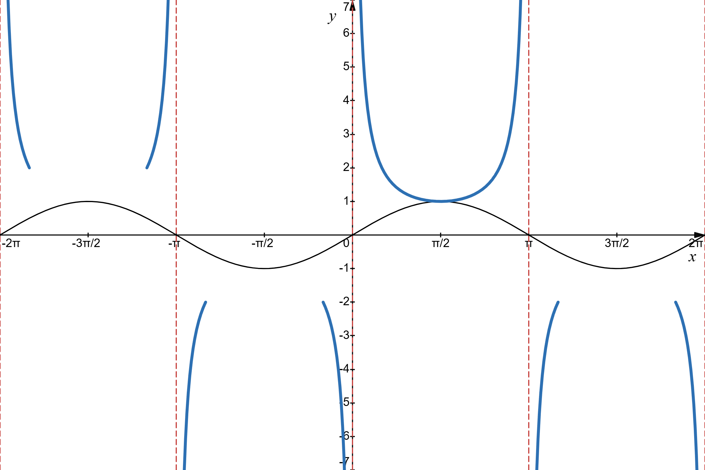
Figure \( \PageIndex{ 6 } \): The base graph of the cosecant, \( y = \csc\left( x \right) \)

I have left a very lightly sketched sine function in this graph. This is because when you are graphing the cosecant, you will inevitably need to start by graphing its reciprocal.

Just as we did with the fundamental trigonometric functions, we now summarize the properties of the cosecant function (with the help of its graph as a visual aid).

Theorem: Properties of \( y = \csc\left( x \right) \)

• Domain: All \( x \ne k \pi \), where \( k \in \mathbb{Z} \)
• Range: \( \left( -\infty, -1 \right] \cup \left[ 1, \infty \right) \)
• Symmetry: Odd (symmetric about the origin)
• Principal Cycle: \( \left[ 0,2\pi \right] \)
• Natural Period: \( 2 \pi \)
• Amplitude: N/A
• Zeros: None

Graphing the Secant Function

The derivation of the graph of the secant function is similar to that of the cosecant function. It is left for you as an exercise.

Theorem: Properties of \( y = \sec\left( x \right) \)

• Domain: All \( x \ne \frac{\pi}{2} + k \pi \), where \( k \in \mathbb{Z} \)
• Range: \( \left( -\infty, -1 \right] \cup \left[ 1, \infty \right) \)
• Symmetry: Even (symmetric about the \( y \)-axis)
• Principal Cycle: \( \left[ 0,2\pi \right] \)
• Natural Period: \( 2 \pi \)
• Amplitude: N/A
• Zeros: None

As with the graph of the cosecant, we usually lightly graph the reciprocal of the secant (which is the cosine) to help us in graphing the secant.

Graphing the Cotangent Function

As with the cosecant and the secant, to graph the cotangent function, we will use its reciprocal. That is, because\[ \cot\left( x \right) = \dfrac{1}{\tan\left( x \right)}, \nonumber \]we will first graph the tangent and discuss what happens as the tangent function tends to zero.

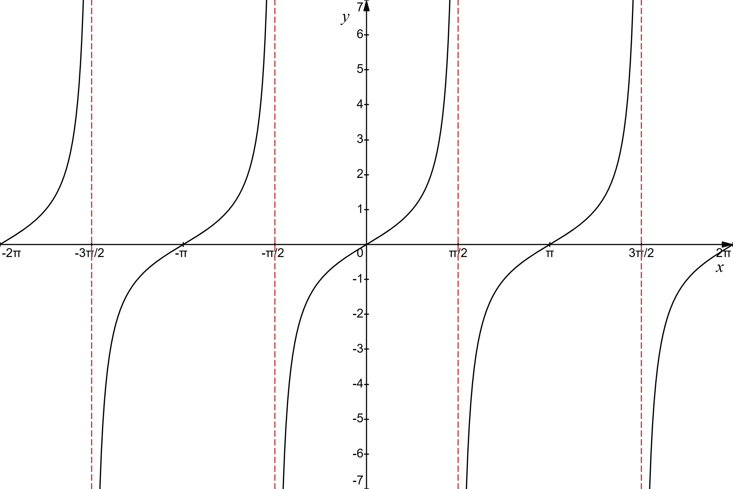
Figure \( \PageIndex{ 7 } \): \( y = \tan\left( x \right) \)

Figure \( \PageIndex{ 7 } \) shows the base graph of the tangent function. Using the same arguments as before, we can get the behavior of the reciprocal function, \( \frac{1}{\tan\left( x \right)} = \cot\left( x \right) \), near the zeros of the tangent.

Figure \( \PageIndex{ 8 } \): Almost done graphing the base graph of the cotangent

Notice in Figure \( \PageIndex{ 8 } \) that the vertical asymptotes are not in the same places as the vertical asymptotes for the tangent. This is because the tangent is undefined when the cosine function is zero (at \( x = \frac{\pi}{2} + k \pi \)) and the cotangent is undefined when the sine is zero (at \( x = k \pi \)). Evaluating the cotangent function for a few special values between \( x=0 \) and \( x = \pi \) should give us the pattern of those missing middle regions.\[ \begin{array}{|c|c|}
\hline x & \cot\left( x \right) \\
\hline \dfrac{\pi}{4} & 1 \\
\hline \dfrac{\pi}{2} & 0 \\
\hline \dfrac{3\pi}{4} & -1 \\
\hline \end{array} \nonumber \]Plotting these points, filling out the rest of the curve with the same pattern, and erasing the underlying tangent graph, we get the following:

Figure \( \PageIndex{ 9 } \): The base graph of the cotangent, \( y = \cot\left( x \right) \)

As before, we list all of the properties in a convenient theorem.

Theorem: Properties of \( y = \cot\left( x \right) \)

• Domain: All \( x \ne k \pi \), where \( k \in \mathbb{Z} \)
• Range: \( \left( -\infty, \infty \right) \)
• Symmetry: Odd (symmetric about the origin)
• Principal Cycle: \( \left[ 0,\pi \right] \)
• Natural Period: \( \pi \)
• Amplitude: N/A
• Zeros: \( x = \frac{\pi}{2} + k \pi \), where \( k \in \mathbb{Z} \)

Transformations of the Reciprocal Functions

Graphing transformations of the reciprocal functions is the same as graphing the transformations of the fundamental trigonometric functions. In fact, to graph transformations of the cosecant and secant functions, we first fully graph the transformations of their related fundamental functions. After that, graphing the transformed cosecant and secant functions is a somewhat trivial move. Let's see this in action.

Example \(\PageIndex{1}\)

Graph a single cycle of each function. State all key characteristics of the graph (including domain, range, period, phase shift, etc.).

1. \( f(x) = -1.2 + 2.8\sec\left( -3x - \frac{\pi}{2} \right) \)
2. \( g(x) = 2 \cot\left( 2x - 2 \right) + 1 \)

Solutions

1. Just as we have done previously, we rewrite it in the better form\[ f(x) = 2.8 \sec\left( -3x - \frac{\pi}{2} \right) - 1.2 \nonumber \]Using the fact that secant is an even function, we clean this up a little more to the following:\[ f(x) = 2.8\sec\left( -\left( 3x + \frac{\pi}{2} \right) \right) - 1.2 = 2.8 \sec\left( 3x + \frac{\pi}{2} \right) - 1.2 \nonumber \]Now that we are finished "preconditioning" the function, it's time we discussed how we are going to graph it. With the secant and cosecant, we perform the intermediate step of graphing their reciprocal functions, the cosine and sine, respectively. So, let's graph\[ y = 2.8\cos\left( 3x + \frac{\pi}{2} \right) - 1.2. \nonumber \]We list out all the essential information.\[ \begin{array}{rclcrcl}
   \hline A & = & 2.8 & \implies & \text{Amplitude} & = & 2.8 \\
   \hline B & = & 3 & \implies & \text{Period} & = & \dfrac{\text{Natural Period}}{B} = \dfrac{2 \pi}{3} \\
   \hline \quad & \quad & \quad & \implies & \text{Step Size} & = & \dfrac{\text{Period}}{4} = \dfrac{2 \pi/3}{4} = \dfrac{\pi}{6} \\
   \hline C & = & \dfrac{\pi}{2} & \implies & \text{Phase Shift} & = & - \dfrac{C}{B} = - \dfrac{\pi/2}{3} = -\dfrac{\pi}{6} \\
   \hline D & = & -1.2 & \implies & \text{Vertical Shift} & = & -1.2 \\
   \hline \end{array} \nonumber \]As usual, we graph and label the midline, label the initial number as the phase shift, and step to the other key numbers using the step size.

   

   Note that the distance between the first and last key number is\[ \left| \dfrac{3\pi}{6} - \left( -\dfrac{\pi}{6} \right) \right| = \dfrac{2\pi}{3} = \text{Period}, \nonumber \]so we have done something right! We then graph the non-reflected cosine, draw in and label the \( y \)-axis, and use that to place the \( x \)-axis.

   

   Now comes the new part. Wherever the cosine function crosses the midline, the original function is undefined. This gives us our vertical asymptotes at \( x = 0 \), \( x = \pm\frac{2\pi}{6} = \frac{\pi}{3} \), \( x = \pm \frac{4\pi}{6} = \frac{2 \pi}{3} \), and so on. Graphing these vertical asymptotes allows us to graph the secant.

   

   Notice that I didn't remove the sketch of the cosine. This is perfectly fine (and some instructors expect you to leave it). Finally, we should state as much about this function as we can. The domain (by looking at our spectacular graph) is all \( x \ne \frac{\pi}{3}k \), where \( k \in \mathbb{Z} \). The range (again, from the graph) is \( \left( -\infty, -4 \right] \cup \left[ 1.6, \infty \right) \).³ The only thing that we cannot state at this point are the zeros of this function (luckily, I didn't ask for them).
2. Before we start, I need to be clear and state that the secant and cosecant functions are the only ones where we must first graph their reciprocal functions. The base graph for the cotangent is simple enough to handle without bothering with the tangent.
   
   Now, there isn't any preconditioning necessary for this function, so we go ahead and jump right into the other stages. Just like the tangent, the cotangent does not have an amplitude and its natural period is \( \pi \).\[ \begin{array}{rclcrcl}
   \hline B & = & 2 & \implies & \text{Period} & = & \dfrac{\text{Natural Period}}{B} = \dfrac{\pi}{2} \\
   \hline \quad & \quad & \quad & \implies & \text{Step Size} & = & \dfrac{\text{Period}}{4} = \dfrac{\pi/2}{4} = \dfrac{\pi}{8} \\
   \hline C & = & -2 & \implies & \text{Phase Shift} & = & - \dfrac{C}{B} = - \dfrac{-2}{2} = 1 \\
   \hline D & = & 1 & \implies & \text{Vertical Shift} & = & 1 \\
   \hline \end{array} \nonumber \]Graphing and labeling the midline, plotting the phase shift as the first key number, and stepping to each subsequent key number using the step size, we get the following:

   

   Because the phase shift was a rational number and the step size was an irrational number, we could not easily add them. Leaving them in the form above is preferred. If you look at the base graph for the cotangent, its principal cycle occurs from \( x = 0 \) to \( x = \pi \). This cycle starts and ends with a vertical asymptote, decreases from left to right, and crosses the midline halfway through. That's precisely what we are going to do here.

   

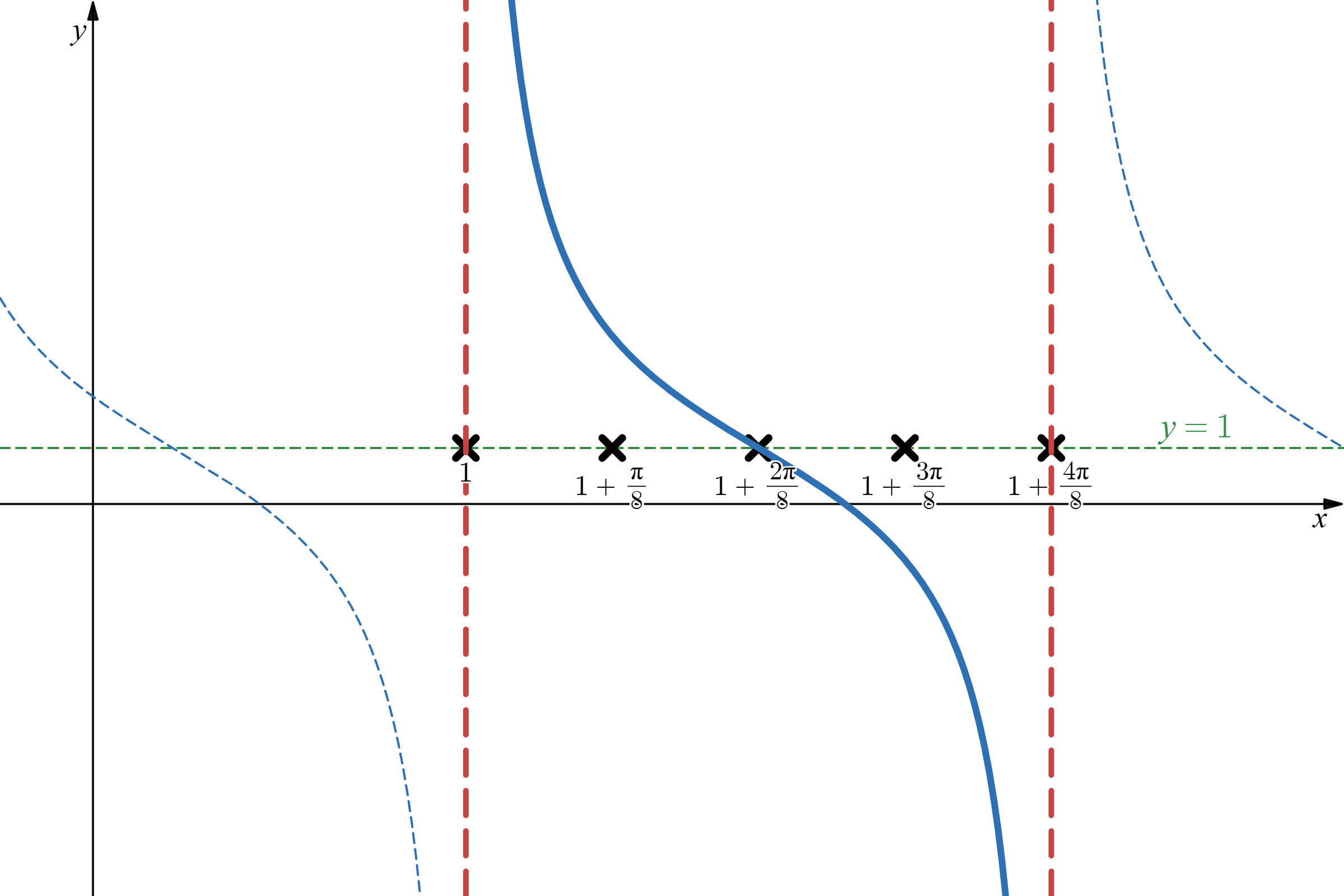
   Now we place the \( y \)-axis one unit to the left of the phase shift and the \( x \)-axis one unit down from the midline. How do I know how far one unit is? It's more of an art of approximation.

   

   Finally, we should label the two points on the curve at \( x=1+\frac{\pi}{8} \) and \( x = 1 + \frac{3\pi}{8} \). The good news is that the \( y \)-values of these points vary from the midline by \( |A| \). Thus, the corresponding \( y \)-values are \( y=1+2=3 \) and \( y = 1-2 =-1 \).

   

   The domain of the function is all \( x \ne 1 + \frac{\pi}{2}k \), where \( k \in \mathbb{Z} \). The range is all real numbers, \( \mathbb{R} \).

Checkpoint \(\PageIndex{1}\)

Graph the function. Clearly state all key information (including domain and range).\[ y = 3 - 4 \csc\left( -\pi x + \dfrac{2}{3}\pi \right) \nonumber \]

Answer

Amplitude of the related sine function: \( 4 \)
Period: \( 2 \)
Step Size: \( \frac{1}{2} \)
Phase Shift: \( \frac{2}{3} \)
Vertical Shift: \( 3 \)
Domain: All \( x \ne \frac{2}{3} + k \), where \( k \in \mathbb{Z} \)
Range: \( \left( -\infty, 1 \right] \cup \left[ 7, \infty \right)\)

Finding Equations Given Graphs

In section 5.3, we found the equations of sine, cosine, and tangent functions given their graphs. We now do the same thing for their reciprocal functions.

Example \(\PageIndex{2}\)

Find the equation of the graphed function.

1. 
2. 

Solutions

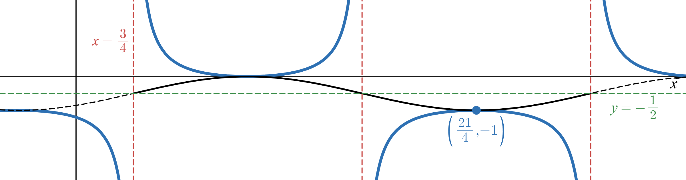
1. As with the sine and cosine functions, graphs of the cosecant and secant are so similar that you could use either as an equation for the given graph (they would just be shifts of one another). A good rule of thumb when building trigonometric equations from graphs is to read the graph from left to right. The piece of information (whether a point or an equation of an asymptote) you have been given will set the beginning of the cycle for the trigonometric function. Therefore, in this case, we will assume the cycle of the trigonometric function starts at \( x = \frac{3}{4} \). With the cosecant and secant, it's beneficial to draw a sinusoid "helper" function. Looking at the given graph, we can see that the midline should be at \( y = -\frac{1}{2} \). Drawing this in allows us to sketch our "helper" function.

   

   We now find the equation of the "helper" function. It is definitely a sine function starting at \( x = \frac{3}{4} \), so the phase shift is\[ -\dfrac{C}{B} = \dfrac{3}{4}.\nonumber \]The midline is \( y = -\frac{1}{2} \), so the vertical shift is\[ D = -\dfrac{1}{2}.\nonumber \]Additionally, the amplitude is the distance between the midline and the maximum or minimum values of the sinusoid. Since the maximum is \( y = 0 \) and the midline is \( y = -\frac{1}{2} \), the amplitude is \( \frac{1}{2} \). Moreover, since this sine function is not reflected,\[ A = \dfrac{1}{2}. \nonumber \]The only thing left to find is the period. This would give us an equation to find \( B \), which in turn would allow us to find \( C \). The cycle begins at \( x = \frac{3}{4} \) and three-quarters of the way through the cycle, we are given the point \( \left( \frac{21}{4},-1 \right) \). That is, the distance between \( \frac{3}{4} \) and \( \frac{21}{4} \) is three-quarters of the period.\[\begin{array}{rrcl}
   & \dfrac{3}{4} \, \text{of the Period} & = & \left| \dfrac{3}{4} - \dfrac{21}{4} \right| \\
   & & = & \left| -\dfrac{18}{4} \right| \\
   & & = & \dfrac{9}{2} \\
   \end{array} \nonumber \]Therefore,\[ \begin{array}{rcl}
   \text{Period} & = & \left( \dfrac{9}{2} \right)\left( \dfrac{4}{3} \right) \\
   & = & 6 \\
   \end{array} \nonumber \]Since the period is \( \frac{2\pi}{B} \),\[ \dfrac{2 \pi}{B} = 6 \implies \dfrac{2 \pi}{6} = B \implies \dfrac{\pi}{3} = B. \nonumber \]Earlier we stated that \( -\frac{C}{B} = \frac{3}{4} \), so\[ -\dfrac{C}{\pi/3} = \dfrac{3}{4} \implies C = - \dfrac{\pi}{4}. \nonumber \]Thus, the "helper" function is\[ y = A \, \sin\left( Bx + C \right) + D = \dfrac{1}{2} \, \sin\left( \dfrac{\pi}{3}x - \dfrac{\pi}{4} \right) - \dfrac{1}{2}. \nonumber \]Finally, the actual function is the reciprocal of the sine. That is, the function in the initial graph is\[ y = \dfrac{1}{2} \, \csc\left( \dfrac{\pi}{3}x - \dfrac{\pi}{4} \right) - \dfrac{1}{2}. \nonumber \]
2. Again, you could write the equation for this in terms of the (reflected) tangent function; however, we will write our equation in terms of the cotangent. Sometimes, you have to "eyeball" the features of a graph. In this example, the midline looks to be \( y = 4 \), so we will say \( D = 4 \). The phase shift could be \( -\frac{\pi}{6} \) or \( +\frac{\pi}{6} \), but the extra point they gave us is in the interval \( \left( -\frac{\pi}{6}, \frac{\pi}{6} \right) \), so we will choose our phase shift to be \( -\frac{\pi}{6} \). This means\[ -\dfrac{C}{B} = -\dfrac{\pi}{6}. \nonumber \]Furthermore, the period is easy to spot on this graph. From vertical asymptote to vertical asymptote, the distance is \( \frac{2\pi}{6} = \frac{\pi}{3} \). Therefore, the period is \( \frac{\pi}{3} \) and, as such,\[ \dfrac{\pi}{B} = \dfrac{\pi}{3} \implies B = 3. \nonumber \]With this, we can find \( C \).\[ -\dfrac{C}{B} = -\dfrac{\pi}{6} \implies \dfrac{C}{3} = \dfrac{\pi}{6} \implies C = \dfrac{\pi}{2}. \nonumber \]We are close to the finish line. Our function is\[ y = A \, \cot\left( 3x + \dfrac{\pi}{2} \right) + 4. \nonumber \]Now we use the given data point to help us find the value of \( A \).\[ \begin{array}{rrcl}
   & 4.1 & = & A \, \cot\left( 3\left( -\dfrac{\pi}{12} \right) + \dfrac{\pi}{2} \right) + 4 \\
   \implies & 0.1 & = & A \, \cot\left( -\dfrac{\pi}{4} + \dfrac{\pi}{2} \right) \\
   \implies & 0.1 & = & A \, \cot\left( \dfrac{\pi}{4} \right) \\
   \implies & 0.1 & = & A \, \left( 1 \right) \\
   \implies & 0.1 & = & A \\
   \end{array} \nonumber \]Thus, the function is\[ y = 0.1 \, \cot\left( 3x + \dfrac{\pi}{2} \right) + 4. \nonumber \]

Checkpoint \(\PageIndex{2}\)

Find the equation of the graphed function.

Answer

\( y = 2\sec\left(3x+\frac{\pi}{5}\right)+1 \)

---

Footnotes

¹ Recall, from section 5.1, the notation \( x \to a^- \) means we are allowing the values of \( x \) to approach \( a \), but from the left side of \( a \). Likewise, \( x \to a^+ \) means \( x \) is approaching \( a \), but from the right side of \( a \). In both cases, we never allow \( x \) to become \( a \).

² This is (hopefully) a skill you have from your prerequisite Algebra course; however, you might be taking this course in Trigonometry prior to taking a course in College Algebra. If this is the case, you will review how to graph rational functions once you take that course.

³ With transformed functions, the graph is the easiest way to find the domain and range. This is a great reason to know how to graph these functions.

---

Homework

Concept Check

1. Describe the general shape of the graph of the cosecant function.

2. What is the relationship between the sine function and the cosecant function? How does this relationship affect their graphs?

3. Describe the general shape of the graph of the secant function.

4. What is the relationship between the cosine function and the secant function? How does this relationship affect their graphs?

5. Describe the general shape of the graph of the cotangent function.

6. What is the relationship between the tangent function and the cotangent function? How does this relationship affect their graphs?

Basic Skills

7. Determine the period, phase shift, and midline of the function \( y = 3 \sec(2x - \pi) + 1 \).

8. Determine the period, phase shift, and midline of the function \( y = 2 \csc(x + \frac{\pi}{4}) - 3 \).

9. Determine the period, phase shift, and midline of the function \( y = -\cot\left(\frac{1}{2}x - \frac{\pi}{3}\right) + 4 \).

10. Determine the period, phase shift, and midline of the function \( y = 4 \sec\left(\frac{1}{3}x + \frac{\pi}{6}\right) - 2 \).

11. Determine the period, phase shift, and midline of the function \( y = -2 \csc(3x - \pi) + 1 \).

12. Determine the period, phase shift, and midline of the function \( y = 3 \cot\left(4x + \frac{\pi}{2}\right) - 5 \).

13. Graph \( y = \sec(x - \frac{\pi}{2}) + 2 \).

14. Graph \( y = 2 \csc\left(\frac{\pi}{2}x\right) - 1 \).

15. Graph \( y = -\cot\left(x + \frac{\pi}{4}\right) + 3 \).

16. Graph \( y = 3 \sec(2x) - 4 \).

17. Graph \( y = -\csc\left(\frac{1}{2}x - \frac{\pi}{3}\right) + 2 \).

18. Graph \( y = \cot\left(\frac{3}{2}x + \frac{\pi}{6}\right) - 1 \).

19. Graph \( y = -2 \sec\left(\frac{1}{3}x - \frac{\pi}{4}\right) + 5 \).

20. Graph \( y = 4 \csc(3x) - 3 \).

21. Graph \( y = \cot(2x) + 4 \).

22. Graph \( y = -\sec\left(\frac{2}{3}x + \frac{\pi}{2}\right) - 2 \).

23. Graph \( y = \csc\left(\frac{\pi}{3}x - \frac{\pi}{6}\right) + 1 \).

24. Graph \( y = -3 \cot\left(\frac{1}{2}x + \frac{\pi}{3}\right) + 2 \).

For Problems 25 - 28, assume that the related sinusoidal function has an amplitude of \( 1 \).

25. Given the graph of a secant function that has a period of \( \pi \), a phase shift of \( \frac{\pi}{4} \) to the right, and a vertical shift up by 2 units, determine the equation of the graph.

26. Given the graph of a cosecant function that has a period of \( 2\pi \), a phase shift of \( \frac{\pi}{6} \) to the left, and a vertical shift down by 3 units, determine the equation of the graph.

27. Given the graph of a reflected secant function that has a period of \( \frac{\pi}{2} \), a phase shift of \( \frac{\pi}{2} \) to the left, and a vertical shift down by 4 units, determine the equation of the graph.

28. Given the graph of a reflected cosecant function that has a period of \( 4\pi \), a phase shift of \( \frac{\pi}{4} \) to the right, and a vertical shift up by 5 units, determine the equation of the graph.

29. Given the graph of a secant function with a period of \( 2\pi \), a vertical shift up by 1 unit, and where the related sinusoidal function has an amplitude of 3, determine the equation of the graph.

30. Given the graph of a cosecant function with a period of \( \pi \), a vertical shift down by 4 units, and where the related sinusoidal function has an amplitude of 2, determine the equation of the graph.

31. Given the graph of a reflected secant function with a period of \( \frac{\pi}{3} \), a phase shift of \( \frac{\pi}{2} \) to the left, a vertical shift down by 3 units, and where the related sinusoidal function has an amplitude of 1.2, determine the equation of the graph.

32. Given the graph of a reflected cosecant function with a period of \( \frac{\pi}{4} \), a phase shift of \( \frac{\pi}{6} \) to the right, a vertical shift up by 2 units, and where the related sinusoidal function has an amplitude of 2, determine the equation of the graph.

For Problems 33 - 35, find the equation of the function in terms of cosecant, secant, or cotangent.

33.  

    

34.  

    

35.  

    

Synthesis Questions

36. Given the function \( y = 3 \csc(2x - \frac{\pi}{2}) + 4 \), find all asymptotes within the interval \( [0, 2\pi] \). Explain the process of identifying these asymptotes.

37. Given the function \( y = 2 \sec\left(\frac{1}{2}x - \frac{\pi}{3}\right) - 1 \), find all asymptotes within the interval \( [-2\pi, 2\pi] \). Describe the method used to determine these asymptotes.

38. For the function \( y = -3 \csc(4x + \frac{\pi}{4}) + 2 \), determine all asymptotes within the interval \( [0, \pi] \). Explain your reasoning and the steps taken to find these asymptotes.

39. Given the function \( y = \sec(3x - \frac{\pi}{6}) - 2 \), find the equations of all vertical asymptotes within the interval \( [-\pi, \pi] \). Describe the procedure used to identify these asymptotes.

40. For the function \( y = -\csc\left(\frac{3}{2}x + \frac{\pi}{3}\right) + 5 \), find the equations of all vertical asymptotes within the interval \( [-\pi, \pi] \). Detail the steps and logic used to locate these asymptotes.

41. Consider the function \( y = 4 \sec\left(2x - \frac{\pi}{2}\right) + 1 \). Identify all vertical asymptotes within the interval \( [0, 2\pi] \) and explain how you determined their locations.