Chapter 6: Analytic Trigonometry

Last updated
Save as PDF

Page ID: 145935

Roy Simpson & Katherine Yoshiwara
Los Angeles Pierce College

$ \newcommand{\vecs}[1]{\overset { \scriptstyle \rightharpoonup} {\mathbf{#1}} } $

$ \newcommand{\vecd}[1]{\overset{-\!-\!\rightharpoonup}{\vphantom{a}\smash {#1}}} $

$ \newcommand{\id}{\mathrm{id}}$ $ \newcommand{\Span}{\mathrm{span}}$

( \newcommand{\kernel}{\mathrm{null}\,}\) $ \newcommand{\range}{\mathrm{range}\,}$

$ \newcommand{\RealPart}{\mathrm{Re}}$ $ \newcommand{\ImaginaryPart}{\mathrm{Im}}$

$ \newcommand{\Argument}{\mathrm{Arg}}$ $ \newcommand{\norm}[1]{\| #1 \|}$

$ \newcommand{\inner}[2]{\langle #1, #2 \rangle}$

$ \newcommand{\Span}{\mathrm{span}}$

$ \newcommand{\id}{\mathrm{id}}$

$ \newcommand{\Span}{\mathrm{span}}$

$ \newcommand{\kernel}{\mathrm{null}\,}$

$ \newcommand{\range}{\mathrm{range}\,}$

$ \newcommand{\RealPart}{\mathrm{Re}}$

$ \newcommand{\ImaginaryPart}{\mathrm{Im}}$

$ \newcommand{\Argument}{\mathrm{Arg}}$

$ \newcommand{\norm}[1]{\| #1 \|}$

$ \newcommand{\inner}[2]{\langle #1, #2 \rangle}$

$ \newcommand{\Span}{\mathrm{span}}$ $ \newcommand{\AA}{\unicode[.8,0]{x212B}}$

$ \newcommand{\vectorA}[1]{\vec{#1}} % arrow$

$ \newcommand{\vectorAt}[1]{\vec{\text{#1}}} % arrow$

$ \newcommand{\vectorB}[1]{\overset { \scriptstyle \rightharpoonup} {\mathbf{#1}} } $

$ \newcommand{\vectorC}[1]{\textbf{#1}} $

$ \newcommand{\vectorD}[1]{\overrightarrow{#1}} $

$ \newcommand{\vectorDt}[1]{\overrightarrow{\text{#1}}} $

$ \newcommand{\vectE}[1]{\overset{-\!-\!\rightharpoonup}{\vphantom{a}\smash{\mathbf {#1}}}} $

$ \newcommand{\vecs}[1]{\overset { \scriptstyle \rightharpoonup} {\mathbf{#1}} } $

$ \newcommand{\vecd}[1]{\overset{-\!-\!\rightharpoonup}{\vphantom{a}\smash {#1}}} $

$\newcommand{\avec}{\mathbf a}$ $\newcommand{\bvec}{\mathbf b}$ $\newcommand{\cvec}{\mathbf c}$ $\newcommand{\dvec}{\mathbf d}$ $\newcommand{\dtil}{\widetilde{\mathbf d}}$ $\newcommand{\evec}{\mathbf e}$ $\newcommand{\fvec}{\mathbf f}$ $\newcommand{\nvec}{\mathbf n}$ $\newcommand{\pvec}{\mathbf p}$ $\newcommand{\qvec}{\mathbf q}$ $\newcommand{\svec}{\mathbf s}$ $\newcommand{\tvec}{\mathbf t}$ $\newcommand{\uvec}{\mathbf u}$ $\newcommand{\vvec}{\mathbf v}$ $\newcommand{\wvec}{\mathbf w}$ $\newcommand{\xvec}{\mathbf x}$ $\newcommand{\yvec}{\mathbf y}$ $\newcommand{\zvec}{\mathbf z}$ $\newcommand{\rvec}{\mathbf r}$ $\newcommand{\mvec}{\mathbf m}$ $\newcommand{\zerovec}{\mathbf 0}$ $\newcommand{\onevec}{\mathbf 1}$ $\newcommand{\real}{\mathbb R}$ $\newcommand{\twovec}[2]{\left[\begin{array}{r}#1 \\ #2 \end{array}\right]}$ $\newcommand{\ctwovec}[2]{\left[\begin{array}{c}#1 \\ #2 \end{array}\right]}$ $\newcommand{\threevec}[3]{\left[\begin{array}{r}#1 \\ #2 \\ #3 \end{array}\right]}$ $\newcommand{\cthreevec}[3]{\left[\begin{array}{c}#1 \\ #2 \\ #3 \end{array}\right]}$ $\newcommand{\fourvec}[4]{\left[\begin{array}{r}#1 \\ #2 \\ #3 \\ #4 \end{array}\right]}$ $\newcommand{\cfourvec}[4]{\left[\begin{array}{c}#1 \\ #2 \\ #3 \\ #4 \end{array}\right]}$ $\newcommand{\fivevec}[5]{\left[\begin{array}{r}#1 \\ #2 \\ #3 \\ #4 \\ #5 \\ \end{array}\right]}$ $\newcommand{\cfivevec}[5]{\left[\begin{array}{c}#1 \\ #2 \\ #3 \\ #4 \\ #5 \\ \end{array}\right]}$ $\newcommand{\mattwo}[4]{\left[\begin{array}{rr}#1 \amp #2 \\ #3 \amp #4 \\ \end{array}\right]}$ $\newcommand{\laspan}[1]{\text{Span}\{#1\}}$ $\newcommand{\bcal}{\cal B}$ $\newcommand{\ccal}{\cal C}$ $\newcommand{\scal}{\cal S}$ $\newcommand{\wcal}{\cal W}$ $\newcommand{\ecal}{\cal E}$ $\newcommand{\coords}[2]{\left\{#1\right\}_{#2}}$ $\newcommand{\gray}[1]{\color{gray}{#1}}$ $\newcommand{\lgray}[1]{\color{lightgray}{#1}}$ $\newcommand{\rank}{\operatorname{rank}}$ $\newcommand{\row}{\text{Row}}$ $\newcommand{\col}{\text{Col}}$ $\renewcommand{\row}{\text{Row}}$ $\newcommand{\nul}{\text{Nul}}$ $\newcommand{\var}{\text{Var}}$ $\newcommand{\corr}{\text{corr}}$ $\newcommand{\len}[1]{\left|#1\right|}$ $\newcommand{\bbar}{\overline{\bvec}}$ $\newcommand{\bhat}{\widehat{\bvec}}$ $\newcommand{\bperp}{\bvec^\perp}$ $\newcommand{\xhat}{\widehat{\xvec}}$ $\newcommand{\vhat}{\widehat{\vvec}}$ $\newcommand{\uhat}{\widehat{\uvec}}$ $\newcommand{\what}{\widehat{\wvec}}$ $\newcommand{\Sighat}{\widehat{\Sigma}}$ $\newcommand{\lt}{<}$ $\newcommand{\gt}{>}$ $\newcommand{\amp}{&}$ $\definecolor{fillinmathshade}{gray}{0.9}$

Mapmakers have always faced an unavoidable challenge: It is impossible to translate the surface of a sphere onto a flat map without some form of distortion. Over the years, a variety of map projections have been developed to suit different uses.

$Screen Shot 2023-01-17 at 12.08.25 AM.png$

The sixteenth century was an age of discovery, when explorers and merchants began sailing to distant and previously unknown lands. But at that time there was no reliable technology for navigation. Although more regions of the world were being mapped more accurately, a flat map by itself was not enough to help a sailor in the middle of the ocean.

In 1569, the Flemish cartographer Gerardus Mercator published a new map using what is known as a cylindrical projection. To imagine how a Mercator projection works, picture shining a light through a glass globe onto a piece of paper rolled into a cylinder and wrapped around the globe. The cylinder is tangent to the globe at its equator.

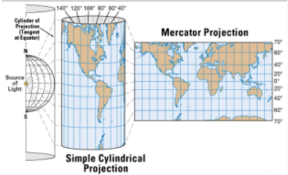
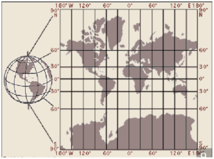
$Screen Shot 2023-01-17 at 12.31.35 AM.png$

Notice how the latitude lines are farther apart the farther you get from the Equator. This projection distorts the size of objects as the latitude increases, so that Greenland and Antarctica appear much larger than they actually are.

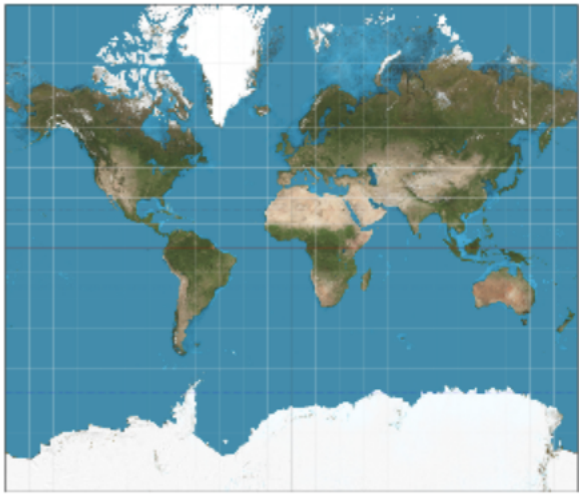
$Screen Shot 2023-01-17 at 12.32.27 AM.png$

But the Mercator projection map is ideally suited for navigation, because any straight line on the map is a line of constant true bearing. If a navigator measures the bearing on the map from his location to his destination, he can set his ship’s compass for the same bearing and maintain that course.

However, the Mercator projection does not preserve distances. On a globe, circles of latitude (also known as parallels) get smaller as they move away from the Equator towards the poles. Thus, in the Mercator projection, when a globe is ”unwrapped” on to a rectangular map, the parallels need to be stretched to the length of the Equator. Mercator had to increase the scale of his map gradually as it moved away from the equator, so that the latitude lines appear equal in length to the equator.

The horizontal scale factor at any latitude must be inversely proportional to lengths on that latitude. Because the radius of the circle of latitude $\theta$ is $R \cos \theta$, the corresponding parallel on the map must be stretched by a factor of $\frac{1}{\cos \theta}$. And because the secant is the reciprocal of the cosine, the scale factor is proportional to the secant of the latitude.

A variety of ”equal area” projections have been developed in modern times, but the Mercator projection is still widely used, in classrooms and atlases. For many people, it represents our image of the world.

$Screen Shot 2023-01-17 at 12.34.33 AM.png$

6.1: Basic Trigonometric Identities and Proof Techniques
This section reviews basic trigonometric identities and proof techniques. It covers Reciprocal, Ratio, Pythagorean, Symmetry, and Cofunction Identities, providing definitions and alternate forms. The section emphasizes understanding over memorization and offers a strategy for proving identities, including steps like simplifying complex expressions, converting to sines and cosines, and working with each side of an equation separately.
6.2: Sum and Difference Identities
This section covers the Sum and Difference Identities for sine, cosine, and tangent. It explains how to use these identities to find the exact values of trigonometric functions at non-special angles, prove equations are identities, and simplify expressions. The section includes detailed examples and exercises for practical application, demonstrating the derivation and usage of these identities in various trigonometric problems.
6.3: Double-Angle Identities
This section covers the Double-Angle Identities for sine, cosine, and tangent, providing formulas and techniques for deriving these identities. It explains how to find exact values for trigonometric functions involving double angles, use these identities in proofs, and apply them in graphing equations. Practical examples and checkpoints illustrate the concepts, helping readers understand and utilize double-angle identities effectively.
6.4: Half-Angle and Power Reduction Identities
This section introduces the Half-Angle and Power Reduction Identities, deriving them from Double-Angle Identities. It explains how to use these identities to rewrite expressions involving trigonometric functions with powers greater than one, and to find exact values of trigonometric functions for half-angles. The section includes practical examples and exercises to illustrate the application of these identities in simplifying trigonometric expressions and solving problems.
6.5: Sum-to-Product and Product-to-Sum Identities
This section covers Sum-to-Product and Product-to-Sum Identities, demonstrating how to convert sums or differences of sines and cosines into products and vice versa. It explains their derivations, provides formulas for these conversions, and includes practical examples for applying these identities in evaluating trigonometric functions and simplifying expressions. These techniques are particularly useful in calculus and other advanced mathematical applications.

Search

Text Color

Text Size

Margin Size

Font Type