3.1: Sequences

Learning Objectives

• Find the formula for the general term of a sequence.
• Calculate the limit of a sequence if it exists.
• Determine the convergence or divergence of a given sequence.

In this section, we reintroduce the concept of sequences that you learned back in Precalculus. The calculus of sequences affords us the opportunity to define what it means for a sequence to converge or diverge. We show how to find limits of sequences that converge, often by using the properties of limits for functions discussed in Calclus I. We close this section with the Monotone Convergence Theorem, a tool we can use to prove that certain types of sequences converge.

---

Terminology of Sequences

To work with this new topic, we need some new terms and definitions. First, an infinite sequence is an ordered list of numbers of the form

\[a_1,a_2,a_3, \ldots ,a_n, \ldots .\nonumber \]

Each of the numbers in the sequence is called a term. The symbol \(n\) is called the index variable for the sequence. We use the notation

\[\{a_n\}^{\infty}_{n=1},\nonumber \]

or simply \(\{a_n\}\), to denote this sequence.¹ Because, in general, a particular number \(a_n\) exists for each positive integer \(n\), we can also define a sequence as a function whose domain is the set of positive integers.

Let’s consider the infinite, ordered list

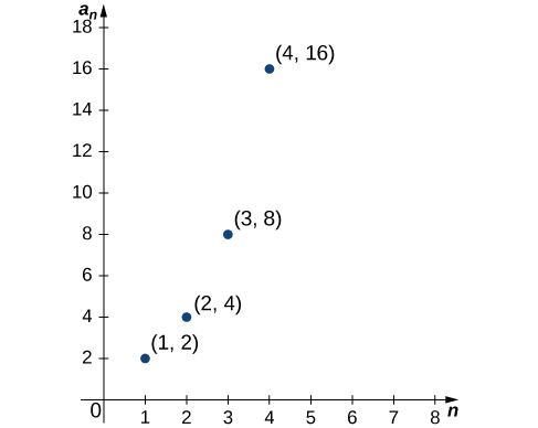
\[2,4,8,16,32, \ldots .\nonumber \]

This is a sequence in which the first, second, and third terms are given by \(a_1=2\), \(a_2=4\), and \(a_3=8\). You can probably see that the terms in this sequence have the following pattern:

\[a_1=2^1,\,a_2=2^2,\,a_3=2^3,\,a_4=2^4 \text{ and } a_5=2^5.\nonumber \]

Assuming this pattern continues, we can write the \(n^{\text{th}}\) term in the sequence by the explicit formula \(a_n=2^n\). Using this notation, we can write this sequence as

\[\{2^n\}^{\infty}_{n=1}, \nonumber \]

or

\[\{2^n\}, \nonumber \]

or

\[a_n = 2^n. \label{explicitformula} \]

The formula in Equation \( \ref{explicitformula} \) is called an explicit formula (or explicit relation) for the sequence.

Alternatively, we can describe this sequence in a different way. Since each term is twice the previous term, this sequence can be defined recursively by expressing the \(n^{\text{th}}\) term, \(a_n\), in terms of the previous term, \(a_{n−1}\). In particular, we can define this sequence as the sequence \(\{a_n\}\) where \(a_1=2\) and, for all \(n \geq 2\), each term \(a_n\) is defined by the recurrence relation

\[a_n=2a_{n−1}. \nonumber \]

In a recurrence relation, one term (or more) of the sequence is given explicitly, and subsequent terms are defined in terms of earlier terms in the sequence.

Note that the index does not have to start at \(n=1\) but could start with other integers. For example, a sequence given by the explicit formula \(a_n=f(n)\) could start at \(n=0\), in which case the sequence would be

\[a_0,\,a_1,\,a_2, \ldots .\nonumber \]

Similarly, for a sequence defined by a recurrence relation, the term \(a_0\) may be given explicitly, and the terms \(a_n\) for \(n \geq 1\) may be defined in terms of \(a_{n−1}\).

The graph of a sequence \(\{a_n\}\) consists of all points \((n,a_n)\) for all positive integers \(n\).² Figure \( \PageIndex{1} \) shows the graph of \({2^n}\).

Figure \(\PageIndex{1}\): The plotted points are a graph of the sequence {\(2^n\)}.

Two types of sequences occur often and are given special names: arithmetic sequences and geometric sequences. In an arithmetic sequence, the difference between every pair of consecutive terms is the same. For example, consider the sequence

\[3,\,7,\,11,\,15,1\,9, \,\ldots . \nonumber \]

You can see that the difference between every consecutive pair of terms is \(4\). Assuming that this pattern continues, this sequence is an arithmetic sequence. It can be described by using the recurrence relation

\[\begin{cases}
a_1 = 3 \\
a_n = a_{n−1}+4, \text{ for } \ n \geq 2
\end{cases}.\nonumber \]

Note that

\[a_2=3+4\nonumber \]

\[a_3=3+4+4=3+2 \cdot 4\nonumber \]

\[a_4=3+4+4+4=3+3 \cdot 4.\nonumber \]

Thus the sequence can also be described using the explicit formula

\[a_n=3+4(n−1)=4n−1.\nonumber \]

In general, an arithmetic sequence is any sequence that can be written in the form \(a_n=cn+b\).

In a geometric sequence, the ratio of every pair of consecutive terms is the same. For example, consider the sequence

\[2,\,−\dfrac{2}{3},\,\dfrac{2}{9},\,−\dfrac{2}{27},\,\dfrac{2}{81}, \ldots .\nonumber \]

We see that the ratio of any term to the preceding term is \(−\frac{1}{3}\). Assuming this pattern continues, this sequence is a geometric sequence. It can be defined recursively as

\[ \begin{cases}
a_1 = 2 \\
a_n =−\dfrac{1}{3} \cdot a_{n−1}, \text{ for }\ n \geq 2.
\end{cases} \nonumber \]

Alternatively, since

\[ \begin{array}{rcl}
a_2 & = & −\dfrac{1}{3} \cdot (2) \\
a_3 & = & \left(−\dfrac{1}{3}\right)\left(−\dfrac{1}{3}\right)(2)=\left(−\dfrac{1}{3}\right)^2 \cdot (2) \\
a_4 & = & \left(−\dfrac{1}{3}\right)\left(−\dfrac{1}{3}\right)\left(−\dfrac{1}{3}\right)(2)=\left(−\dfrac{1}{3}\right)^3 \cdot (2), \\
\end{array} \nonumber \]

we see that the sequence can be described by using the explicit formula³

\[a_n=2 \left(−\dfrac{1}{3}\right)^{n−1}.\nonumber \]

The sequence \(\{2^n\}\) that we discussed earlier is a geometric sequence, where the ratio of any term to the previous term is \(2\). In general, a geometric sequence is any sequence that can be written in the form \(a_n = c r^n\).

Example \(\PageIndex{1}\): Finding Explicit Formulas

For each of the following sequences, find an explicit formula for the \(n^{\text{th}}\) term of the sequence.

1. \(−\frac{1}{2},\frac{2}{3},−\frac{3}{4},\frac{4}{5},−\frac{5}{6}, \ldots \)
2. \(\frac{3}{4},\frac{9}{7},\frac{27}{10},\frac{81}{13},\frac{243}{16}, \ldots \).

Solution

a. First, note that the sequence is alternating from negative to positive. The odd terms in the sequence are negative, and the even terms are positive. Therefore, the \(n^{\text{th}}\) term includes a factor of \((−1)^n\). Next, consider the sequence of numerators \({1,2,3, \ldots }\) and the sequence of denominators \({2,3,4, \ldots }\). We can see that both of these sequences are arithmetic sequences. The \(n^{\text{th}}\) term in the sequence of numerators is \(n\), and the \(n^{\text{th}}\) term in the sequence of denominators is \(n+1\). Therefore, the sequence can be described by the explicit formula

\[a_n=\dfrac{(−1)^nn}{n+1}. \nonumber \]

b. The sequence of numerators \(3,9,27,81,243, \ldots \) is a geometric sequence. The numerator of the \(n^{\text{th}}\) term is \(3^n\). The sequence of denominators \(4,7,10,13,16, \ldots \) is an arithmetic sequence. The denominator of the \(n^{\text{th}}\) term is \(4+3(n−1)=3n+1\). Therefore, we can describe the sequence by the explicit formula

\[a_n=\dfrac{3^n}{3n+1}. \nonumber \]

Exercise \(\PageIndex{1}\)

Find an explicit formula for the \(n^{\text{th}}\) term of the sequence \(\left\{\frac{1}{5},−\frac{1}{7},\frac{1}{9},−\frac{1}{11}, \ldots \right\}.\)

Hint

The denominators form an arithmetic sequence.

Answer

\(a_n=\dfrac{(−1)^{n+1}}{3+2n}\)

Example \(\PageIndex{2}\): Defined by Recurrence Relations

For each of the following recursively defined sequences, find an explicit formula for the sequence.

1. \(a_1=2, a_n=−3a_{n−1}\) for \(n \geq 2\)
2. \(a_1=\left(\frac{1}{2}\right), a_n=a_{n−1}+\left(\frac{1}{2}\right)^n\) for \(n \geq 2\)

Solution

a. Writing out the first few terms, we have

\[ \begin{array}{rcl}
a_1 & = & 2 \\
a_2 & = & −3a_1=−3(2) \\
a_3 & = & −3a_2=(−3)^2 (2) \\
a_4 & = & −3a_3=(−3)^3 (2). \\
\end{array}\]

In general,

\[a_n=2(−3)^{n−1}. \nonumber \]

b. Write out the first few terms:

\[ \begin{array}{rcl}
a_1 & = & \dfrac{1}{2} \\
a_2 & = & a_1+\left(\dfrac{1}{2}\right)^2=\dfrac{1}{2}+\dfrac{1}{4}=\dfrac{3}{4} \\
a_3 & = & a_2+\left(\dfrac{1}{2}\right)^3=\dfrac{3}{4}+\dfrac{1}{8}=\dfrac{7}{8} \\
a_4 & = & a_3+\left(\dfrac{1}{2}\right)^4=\dfrac{7}{8}+\dfrac{1}{16}=\dfrac{15}{16}. \\
\end{array} \nonumber \]

From this pattern, we derive the explicit formula

\[a_n=\dfrac{2^n−1}{2^n}=1−\dfrac{1}{2^n}. \nonumber \]

Exercise \(\PageIndex{2}\)

Find an explicit formula for the sequence defined recursively such that \(a_1=−4\) and \(a_n=a_{n−1}+6\).

Hint

This is an arithmetic sequence.

Answer

\(a_n=6n−10\)

Subsection Footnotes

¹ A similar notation is used for sets, but a sequence is an ordered list, whereas a set is not ordered.

² Remember, the domain of a sequence, in general, is the set of natural numbers (also called the positive integers). As such, the graph of a sequence will not be continuous.

³ Since pattern recognition is an important skill when working with sequences (and it's sister-subject, series), it is often best to not simplify your arithmetic when writing out computations. This allows you to see the "hidden" patterns that make the sequence simple to write in a succinct form.

---

Limit of a Sequence

A fundamental question that arises regarding infinite sequences is the behavior of the terms as \(n\) gets larger. Since a sequence is a function defined on the positive integers, it makes sense to discuss the limit of the terms as \(n \to \infty \). For example, consider the following four sequences and their different behaviors as \(n \to \infty \) (Figure \(\PageIndex{2}\)):

1. \(\{1+3n\}=\{4,7,10,13, \ldots \}\). The terms \(1+3n\) become arbitrarily large as \(n \to \infty \). In this case, we say that \(1+3n \to \infty \) as \(n \to \infty\).
2. \(\left\{1− \left(\frac{1}{2}\right) ^n\right\}=\left\{ \frac{1}{2} ,\frac{3}{4},\frac{7}{8},\frac{15}{16}\, \ldots \right\}\). The terms \(1−\left(\frac{1}{2}\right)^n \to 1\) as \(n \to \infty \).
3. \(\{(−1)^n\}=\{−1,1,−1,1, \ldots \}\). The terms alternate but do not approach one single value as \(n \to \infty\).
4. \(\left\{\frac{(−1)^n}{n}\right\}=\left\{−1,\frac{1}{2},−\frac{1}{3},\frac{1}{4}, \ldots \right\}\). The terms alternate for this sequence as well, but \(\frac{(−1)^n}{n} \to 0\) as \(n \to \infty \).

Figure \(\PageIndex{2}\): (a) The terms in the sequence become arbitrarily large as \(n \to \infty \). (b) The terms in the sequence approach \(1\) as \(n \to \infty \). (c) The terms in the sequence alternate between \(1\) and \(−1\) as \(n \to \infty \). (d) The terms in the sequence alternate between positive and negative values but approach \(0\) as \(n \to \infty \).

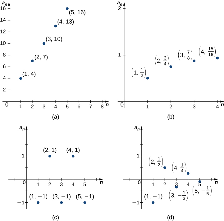
From these examples, we see several possibilities for the behavior of the terms of a sequence as \(n \to \infty \). In two of the sequences, the terms approach a finite number as \(n \to \infty\). In the other two sequences, the terms do not. If the terms of a sequence approach a finite number \(L\) as \(n \to \infty \), we say that the sequence is a convergent sequence and the real number \(L\) is the limit of the sequence. We can give an informal definition here.

Definition: The Informal Definition of the Limit of a Sequence

Given a sequence \(\{a_n\}\), if the terms \(a_n\) become arbitrarily close to a finite number \(L\) as \(n\) becomes sufficiently large, we say \(\{a_n\}\) is a convergent sequence and \(L\) is the limit of the sequence. In this case, we write

\[\lim_{n \to \infty }a_n=L. \nonumber \]

If a sequence \(\{a_n\}\) is not convergent, we say it is a divergent sequence.

From Figure \( \PageIndex{2} \)(b), we see that the terms in the sequence \(\left\{1− \left(\frac{1}{2}\right)^n\right\}\) are becoming arbitrarily close to \(1\) as \(n\) becomes very large. We conclude that \(\left\{1−\left(\frac{1}{2}\right)^n\right\}\) is a convergent sequence and its limit is \(1\). In contrast, from Figure \( \PageIndex{2} \)(a), we see that the terms in the sequence \(1+3n\) are not approaching a finite number as \(n\) becomes larger. We say that \(\{1+3n\}\) is a divergent sequence.

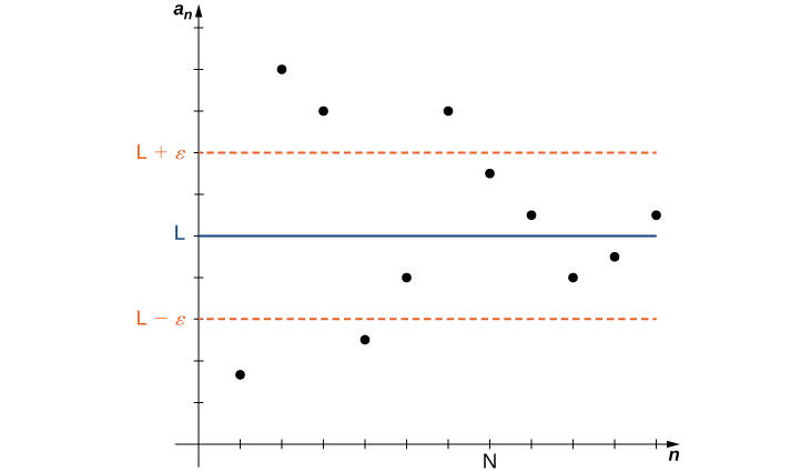
In the informal definition for the limit of a sequence, we used the terms "arbitrarily close" and "sufficiently large." Although these phrases help illustrate the meaning of a converging sequence, they are somewhat vague. To be more precise, we now present the more formal definition of limit for a sequence and show these ideas graphically in Figure \( \PageIndex{2} \).

Definition: The Precise Definition of the Limit of a Sequence

A sequence \(\{a_n\}\) converges to a real number \(L\) if for all \( \epsilon \gt 0\), there exists an integer \(N\) such that for all \(n \geq N\), \(|a_n−L| \lt \epsilon \). The number \(L\) is the limit of the sequence and we write

\[\lim_{n \to \infty }a_n = L \text{ or } a_n \to L. \nonumber \]

In this case, we say the sequence \(\{a_n\}\) is a convergent sequence. If a sequence does not converge, it is a divergent sequence, and we say the limit does not exist.⁴

Figure \( \PageIndex{3} \) illustrates the precise definition of the limit of a convergent sequence.

Figure \(\PageIndex{3}\): As \(n\) increases, the terms \(a_n\) become closer to \(L\). For values of \(n \geq N\), the distance between each point \((n,a_n)\) and the line \(y=L\) is less than \( \epsilon \).

We remark that the convergence or divergence of a sequence \(\{a_n\}\) depends only on what happens to the terms \(a_n\) as \(n \to \infty \). Therefore, if a finite number of terms \(b_1,b_2, \ldots ,b_N\) are placed before \(a_1\) to create a new sequence

\[b_1,\,b_2,\, \ldots ,\,b_N,\,a_1,\,a_2,\, \ldots ,\nonumber \]

this new sequence will converge if \(\{a_n\}\) converges and diverge if \(\{a_n\}\) diverges. Furthermore, if the sequence \(\{a_n\}\) converges to \(L\), this new sequence will also converge to \(L\).

As defined above, if a sequence does not converge, it is said to be a divergent sequence. For example, the sequences \(\{1+3n\}\) and \(\left\{(−1)^n\right\}\) shown in Figure \( \PageIndex{2} \) diverge. However, different sequences can diverge in different ways. The sequence \(\left\{(−1)^n\right\}\) diverges because the terms alternate between \(1\) and \(−1\), but do not approach one value as \(n \to \infty \). On the other hand, the sequence \(\{1+3n\}\) diverges because the terms \(1+3n \to \infty \) as \(n \to \infty \). We say the sequence \(\{1+3n\}\) diverges to infinity and write \(\displaystyle \lim_{n \to \infty }(1+3n)= \infty \). It is important to recognize that this notation does not imply the limit of the sequence \(\{1+3n\}\) exists. The sequence is, in fact, divergent. Writing that the limit is infinity is intended only to provide more information about why the sequence is divergent. A sequence can also diverge to negative infinity. For example, the sequence \(\{−5n+2\}\) diverges to negative infinity because \(−5n+2 \to − \infty \) as \(n \to \infty \). We write this as \(\displaystyle \lim_{n \to \infty }(−5n+2) = − \infty\).

Because a sequence is a function whose domain is the set of positive integers, we can use properties of limits of functions to determine whether a sequence converges. For example, consider a sequence \(\{a_n\}\) and a related function \(f\) defined on all positive real numbers such that \(f(n)=a_n\) for all integers \(n \geq 1\). Since the domain of the sequence is a subset of the domain of \(f\), if \(\displaystyle \lim_{x \to \infty }f(x)\) exists, then the sequence converges and has the same limit. For example, consider the sequence \(\left\{\frac{1}{n}\right\}\) and the related function \(f(x)=\frac{1}{x}\). Since the function \(f\) defined on all real numbers \(x \gt 0\) satisfies \(f(x)=\frac{1}{x} \to 0\) as \(x \to \infty \), the sequence \(\left\{\frac{1}{n}\right\}\) must satisfy \(\frac{1}{n} \to 0\) as \(n \to \infty\). We summarize this result as a theorem.

Theorem \( \PageIndex{1} \)

Consider a sequence \(\{a_n\}\) such that \(a_n=f(n)\) for all \(n \geq 1\). If there exists a real number \(L\) such that

\[\lim_{x \to \infty }f(x)=L, \nonumber \]

then \(\{a_n\}\) converges and

\[\lim_{n \to \infty }a_n=L. \nonumber \]

Caution

In general, the converse of Theorem \( \PageIndex{1} \) is not true. For example, consider the sequence \( \{ \sin(\pi n) \} \). For all integer values of \( n \), the value of this sequence is \( 0 \). Hence, \( \displaystyle \lim_{n \to \infty} \sin(\pi n) = 0 \); however, from our work in Calculus I, we know that \( \displaystyle \lim_{x \to \infty} \sin(\pi x) \) does not exist.

It's best to think of Theorem \( \PageIndex{1} \) as follows,

If the infinite limit of the related function exists (and is finite), then the sequence converges (to the same value).

We can use this theorem to evaluate \(\displaystyle \lim_{n \to \infty }r^n\) for \(0 \leq r \leq 1\). For example, consider the sequence \(\left\{(1/2)^n\right\}\) and the related exponential function \(f(x)=(1/2)^x\). Since \(\displaystyle \lim_{x \to \infty }(1/2)^x=0\), we conclude that the sequence \(\left\{(1/2)^n\right\}\) converges and its limit is \(0\). Similarly, for any real number \(r\) such that \(0 \leq r \lt 1\), \(\displaystyle \lim_{x \to \infty }r^x=0\), and therefore the sequence \(\left\{r^n\right\}\) converges (to \( 0 \)). On the other hand, if \(r=1\), then \(\displaystyle \lim_{x \to \infty }r^x=1\), and therefore the limit of the sequence \(\left\{1^n\right\}\) is \(1\). If \(r \gt 1\), \(\displaystyle \lim_{x \to \infty }r^x= \infty \), and therefore we cannot apply this theorem. However, in this case, just as the function \(r^x\) grows without bound as \(n \to \infty \), the terms \(r^n\) in the sequence become arbitrarily large as \(n \to \infty \), and we conclude that the sequence \(\left\{r^n\right\}\) diverges to infinity if \(r \gt 1\).

We summarize these results regarding the geometric sequence \({r^n}\):

\[ \begin{array}{rclcr}
r^n & \to & 0 & \text{if} & 0 \lt r \lt 1 \\
r^n & \to & 1 & \text{if} & r=1 \\
r^n & \to & \infty & \text{if} & r \gt 1 \\
\end{array} \nonumber \]

Later in this section we consider the case when \(r \lt 0\).

We now consider slightly more complicated sequences. For example, consider the sequence \(\left\{(2/3)^n+(1/4)^n\right\}\). The terms in this sequence are more complicated than other sequences we have discussed, but luckily the limit of this sequence is determined by the limits of the two sequences \(\left\{(2/3)^n\right\}\) and \(\left\{(1/4)^n\right\}\). As we describe in the following algebraic Limit Laws, since \(\left\{(2/3)^n\right\}\) and \(\left\{1/4)^n\right\}\) both converge to \(0\), the sequence \(\left\{(2/3)^n+(1/4)^n\right\}\) converges to \(0+0=0\). Just as we were able to evaluate a limit involving an algebraic combination of functions \(f\) and \(g\) by looking at the limits of \(f\) and \(g\) in Calculus I, we are able to evaluate the limit of a sequence whose terms are algebraic combinations of \(a_n\) and \(b_n\) by evaluating the limits of \(\{a_n\}\) and \(\{b_n\}\).

Theorem: Algebraic Limit Laws

Given sequences \(\{a_n\}\) and \(\{b_n\}\) and any real number \(c\), if there exist constants \(A\) and \(B\) such that \(\displaystyle \lim_{n \to \infty }a_n=A\) and \(\displaystyle \lim_{n \to \infty }b_n=B\), then

1. \(\displaystyle \lim_{n \to \infty } c = c\)
2. \(\displaystyle \lim_{n \to \infty }c a_n = c \lim_{n \to \infty }a_n=cA\)
3. \(\displaystyle \lim_{n \to \infty }(a_n \pm b_n)=\lim_{n \to \infty }a_n \pm \lim_{n \to \infty }b_n=A \pm B\)
4. \(\displaystyle \lim_{n \to \infty }(a_n \cdot b_n)=\big(\lim_{n \to \infty }a_n\big) \cdot \big(\lim_{n \to \infty }b_n\big)=A \cdot B\)
5. \(\displaystyle \lim_{n \to \infty }\left(\dfrac{a_n}{b_n}\right)=\dfrac{\displaystyle \lim_{n \to \infty }a_n}{\displaystyle \lim_{n \to \infty }b_n}=\dfrac{A}{B}\), provided \(B \neq 0\) and each \(b_n \neq 0.\)

Proof of part iii.

Let \( \epsilon \gt 0\). Since \(\displaystyle \lim_{n \to \infty }a_n=A\), there exists a constant positive integer \(N_1\) such that \( |a_n - A | \lt \frac{\epsilon}{2} \) for all \(n \geq N_1\). Since \(\displaystyle \lim_{n \to \infty }b_n=B\), there exists a constant \(N_2\) such that \(|b_n−B| \lt \epsilon /2\) for all \(n \geq N_2\). Let \(N = \max\{ N_1, N_2 \}\). Therefore, for all \(n \geq N\), \(|(a_n+b_n)−(A+B)| \leq |a_n−A|+|b_n−B| \lt \frac{ \epsilon }{2}+\frac{ \epsilon }{2}= \epsilon \).

The Algebraic Limit Laws allow us to evaluate limits for many sequences. For example, consider the sequence \(a_n={\frac{1}{n^2}}\). As shown earlier, \(\displaystyle \lim_{n \to \infty }\frac{1}{n}=0\). Similarly, for any positive integer \(k\), we can conclude that

\[\lim_{n \to \infty }\dfrac{1}{n^k}=0. \nonumber \]

In the next example, we make use of this fact along with the Algebraic Limit Laws to evaluate limits for other sequences.

Example \(\PageIndex{3}\): Determining Convergence and Finding Limits

For each of the following sequences, determine whether or not the sequence converges. If it converges, find its limit.

1. \(\left\{5−\frac{3}{n^2}\right\}\)
2. \(\left\{\frac{3n^4−7n^2+5}{6−4n^4}\right\}\)
3. \(\left\{\frac{2^n}{n^2}\right\}\)
4. \(\left\{\left(1+\frac{4}{n}\right)^n\right\}\)

Solution

a. We know that \(\displaystyle \lim_{n \to \infty }\frac{1}{n}=0\). Using this fact, we conclude that

\[\lim_{n \to \infty }\dfrac{1}{n^2}=\lim_{n \to \infty }\dfrac{1}{n} \cdot \lim_{n \to \infty }\dfrac{1}{n}=0. \nonumber \]

Therefore,

\[ \lim_{n \to \infty }\left(5−\dfrac{3}{n^2}\right)=\lim_{n \to \infty }5−3\lim_{n \to \infty }\dfrac{1}{n^2}=5−3.0=5. \nonumber \]

The sequence converges and its limit is \(5\).

b. By factoring \(n^4\) out of the numerator and denominator and using the Algebraic Limit Laws above, we have

\[\begin{array}{rcl}
\displaystyle \lim_{n \to \infty }\dfrac{3n^4−7n^2+5}{6−4n^4} & = & \displaystyle \lim_{n \to \infty }\dfrac{3−\dfrac{7}{n^2}+\dfrac{5}{n^4}}{\dfrac{6}{n^4}−4} \\
& = & \dfrac{\displaystyle \lim_{n \to \infty }(3−\dfrac{7}{n^2}+\dfrac{5}{n^4})}{\displaystyle \lim_{n \to \infty }(\dfrac{6}{n^4}−4)} \\
& = & \dfrac{\displaystyle \lim_{n \to \infty }(3) − \displaystyle \lim_{n \to \infty }\dfrac{7}{n^2} + \displaystyle \lim_{n \to \infty }\dfrac{5}{n^4}}{\displaystyle \lim_{n \to \infty }\dfrac{6}{n^4}−\displaystyle \lim_{n \to \infty }(4)}\\
& = & \dfrac{\displaystyle \lim_{n \to \infty }(3)−7 \cdot \displaystyle \lim_{n \to \infty }\dfrac{1}{n^2}+5 \cdot \displaystyle \lim_{n \to \infty }\dfrac{1}{n^4}}{6 \cdot \displaystyle \lim_{n \to \infty }\dfrac{1}{n^4}−\displaystyle \lim_{n \to \infty }(4)}\\
& = & \dfrac{3−7 \cdot 0+5 \cdot 0}{6 \cdot 0−4} \\
& = & −\dfrac{3}{4}. \\
\end{array} \nonumber \]

The sequence converges and its limit is \(−3/4\).

c. Consider the related function \(f(x)=2^x/x^2\) defined on all real numbers \(x \gt 0\). Since \(2^x \to \infty \) and \(x^2 \to \infty \) as \(x \to \infty \), apply l’Hospital’s Rule and write

\[\begin{array}{rcl}
\displaystyle \lim_{x \to \infty }\dfrac{2^x}{x^2} & \overset{\text{L.R.}}{=} & \displaystyle \lim_{x \to \infty }\dfrac{2^x \ln2}{2x} \\
& \overset{\text{L.R.}}{=} & \displaystyle \lim_{x \to \infty }\dfrac{2^x(\ln2)^2}{2} \\
& = & \infty . \\
\end{array} \nonumber \]

We conclude that the sequence diverges.

d. Consider the function \(f(x)=\left(1+\frac{4}{x}\right)^x\) defined on all real numbers \(x \gt 0\). We start by letting

\[y= \left(1+\dfrac{4}{x}\right)^x. \nonumber \]

Hence,

\[ \begin{array}{rclr}
\ln(y) & = & \ln\left[ \left(1+\dfrac{4}{x}\right)^x \right] & \\
& = & x \ln\left(1+\dfrac{4}{x}\right) & \left( \text{Properties of Logarithms} \right) \\
\end{array} \nonumber \]

Taking the limit of both sides, we get

\[ \begin{array}{rclr}
\displaystyle \lim_{x \to \infty} \ln(y) & = & \displaystyle \lim_{x \to \infty} x \ln\left(1+\dfrac{4}{x}\right) & \\
& = & \displaystyle \lim_{x \to \infty} \dfrac{\ln\left(1+\dfrac{4}{x}\right)}{\frac{1}{x}} & \left( \text{getting the logarithm into an indeterminate form }\frac{0}{0} \right) \\
& \overset{\text{L.R.}}{=} & \displaystyle \lim_{x \to \infty} \dfrac{4}{1+4/x} \\
& = & 4 \\
\end{array} \nonumber \]

Hence,

\[ \begin{array}{rcl}
\displaystyle \lim_{x \to \infty} \left(1+\frac{4}{x}\right)^x & = & \displaystyle \lim_{x \to \infty} y \\
& = & \displaystyle \lim_{x \to \infty} e^{\ln(y)} \\
& = & e^{\displaystyle \lim_{x \to \infty} \ln(y)} \\
& = & e^4 \\
\end{array} \nonumber \]

Hence, since \(\displaystyle \lim_{x \to \infty }\left(1+\frac{4}{x}\right)^x=e^4\), we can conclude that the sequence \(\left\{\left(1+\frac{4}{n}\right)^n\right\}\) converges to \(e^4\).

Exercise \(\PageIndex{3}\)

Consider the sequence \(\left\{(5n^2+1)/e^n\right\}\). Determine whether or not the sequence converges. If it converges, find its limit.

Hint

Use l’Hospital’s Rule.

Answer

The sequence converges, and its limit is \(0\)

Recall that if \(f\) is a continuous function at a value \(L\), then \(f(x) \to f(L)\) as \(x \to L\). This idea applies to sequences as well. Suppose a sequence \(a_n \to L\), and a function \(f\) is continuous at \(L\). Then \(f(a_n) \to f(L)\). This property often enables us to find limits for complicated sequences. For example, consider the sequence \(\sqrt{5−\frac{3}{n^2}}\). From Example \( \PageIndex{3} \)a. we know the sequence \(5−\frac{3}{n^2} \to 5\). Since \(\sqrt{x}\) is a continuous function at \(x=5\),

\[\lim_{n \to \infty }\sqrt{5−\dfrac{3}{n^2}}=\sqrt{\lim_{n \to \infty }(5−\dfrac{3}{n^2})}=\sqrt{5}.\nonumber \]

Theorem \(\PageIndex{2}\)

Consider a sequence \(\{a_n\}\) and suppose there exists a real number \(L\) such that the sequence \(\{a_n\}\) converges to \(L\). Suppose \(f\) is a continuous function at \(L\). Then there exists an integer \(N\) such that \(f\) is defined at all values an for \(n \geq N\), and the sequence \(\{f(a_n)\}\) converges to \(f(L)\) (see Figure \(\PageIndex{4}\)).

Proof

Let \(\epsilon \gt 0\). Since \(f\) is continuous at \(L\), there exists \( \delta \gt 0\) such that \(|f(x)−f(L)| \lt \epsilon \) if \(|x−L|< \delta \). Since the sequence \(\{a_n\}\) converges to \(L\), there exists \(N\) such that \(|a_n−L|< \delta \) for all \(n \geq N\). Therefore, for all \(n \geq N\), \(|a_n−L|< \delta \), which implies \(|f(a_n)−f(L)|< \epsilon \). We conclude that the sequence \(\{f(a_n)\}\) converges to \(f(L)\).

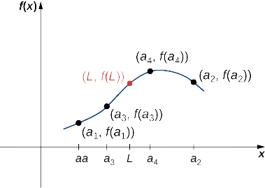
Figure \(\PageIndex{4}\): Because \(f\) is a continuous function as the inputs \(a_1,\,a_2,\,a_3,\, \ldots \) approach \(L\), the outputs \(f(a_1),\,f(a_2),\,f(a_3),\, \ldots \) approach \(f(L)\).

Example \(\PageIndex{4}\): Limits Involving Continuous Functions Defined on Convergent Sequences

Determine whether the sequence \(\left\{\cos(3/n^2)\right\}\) converges. If it converges, find its limit.

Solution

Since the sequence \(\left\{3/n^2\right\}\) converges to \(0\) and \(\cos x\) is continuous at \(x=0\), we can conclude that the sequence \(\left\{\cos(3/n^2)\right\}\) converges and

\[ \lim_{n \to \infty }\cos\left(\dfrac{3}{n^2}\right)=\cos 0=1. \nonumber \]

Exercise \(\PageIndex{4}\)

Determine if the sequence \(\left\{\sqrt{\frac{2n+1}{3n+5}}\right\}\) converges. If it converges, find its limit.

Hint

Consider the sequence \(\left\{\frac{2n+1}{3n+5}\right\}.\)

Answer

The sequence converges, and its limit is \(\sqrt{2/3}\).

Another theorem involving limits of sequences is an extension of the Squeeze Theorem for limits discussed in Calculus I.

Theorem: Squeeze Theorem for Sequences

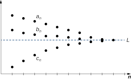
Consider sequences \(\{a_n\}\), \(\{b_n\}\), and \(\{c_n\}\). Suppose there exists an integer \(N\) such that

\[a_n \leq b_n \leq c_n \, \text{for all} \, n \geq N. \nonumber \]

If there exists a real number \(L\) such that

\[\lim_{n \to \infty }a_n=L=\lim_{n \to \infty }c_n, \nonumber \]

then \(\{b_n\}\) converges and \(\displaystyle \lim_{n \to \infty }b_n=L\) (see Figure \(\PageIndex{5}\)).

Figure \(\PageIndex{5}\): Each term bn satisfies \(a_n \leq b_n \leq c_n\) and the sequences \(\{a_n\}\) and \(\{c_n\}\) converge to the same limit, so the sequence \(\{b_n\}\) must converge to the same limit as well.

Proof

Let \( \epsilon \gt 0\). Since the sequence \(\{a_n\}\) converges to \(L\), there exists an integer \(N_1\) such that \(|a_n−L| \lt \epsilon \) for all \(n \geq N_1\). Similarly, since \(\{c_n\}\) converges to \(L\), there exists an integer \(N_2\) such that \(|c_n−L| \lt \epsilon \) for all \(n \geq N_2\). By assumption, there exists an integer \(N\) such that \(a_n \leq b_n \leq c_n\) for all \(n \geq N\). Let \(M = \max\{ N_1, N_2, N \}\). We must show that \(|b_n−L| \lt \epsilon \) for all \(n \geq M\).

For all \(n \geq M\),\[− \epsilon \lt −|a_n−L| \leq a_n−L \leq b_n−L \leq c_n−L \leq |c_n−L| \lt \epsilon. \nonumber \]Therefore, \(− \epsilon \lt b_n−L \lt \epsilon\), and we conclude that \(|b_n−L| \lt \epsilon \) for all \(n \geq M\), and we conclude that the sequence \({b_n}\) converges to \(L\).

Example \(\PageIndex{5}\): Using the Squeeze Theorem

Use the Squeeze Theorem to find the limit of each of the following sequences.

1. \(\left\{\frac{\cos\, n}{n^2}\right\}\)
2. \(\left\{\left(−\frac{1}{2}\right)^n\right\}\)

Solution

a. Since \(−1 \leq \cos n \leq 1\) for all integers \(n\), we have

\[−\dfrac{1}{n^2} \leq \dfrac{\cos n}{n^2} \leq \dfrac{1}{n^2}. \nonumber \]

Since \(−1/n^2 \to 0\) and \(1/n^2 \to 0\) as \( n \to \infty \), we conclude that \(\cos n/n^2 \to 0\) by the Squeeze Theorem.

b. Since

\[−\dfrac{1}{2^n} \leq \left(−\dfrac{1}{2}\right)^n \leq \dfrac{1}{2^n} \nonumber \]

for all positive integers \(n, \, −1/2^n \to 0\) and \(1/2^n \to 0\) as \( n \to \infty \), we can conclude that \((−1/2)^n \to 0\) by the Squeeze Theorem.

Exercise \(\PageIndex{5}\)

Find \(\displaystyle \lim_{n \to \infty }\frac{2n−\sin\, n}{n}.\)

Hint

Use the fact that \(−1 \leq \sin n \leq 1.\)

Answer

\(2\)

Using the idea from Example \(\PageIndex{5}\)b we conclude that \(r^n \to 0\) for any real number \(r\) such that \(−1 \lt r \lt 0\). If \(r \lt −1\), the sequence \({r^n}\) diverges because the terms oscillate and become arbitrarily large in magnitude. If \(r=−1\), the sequence \({r^n}={(−1)^n}\) diverges, as discussed earlier. Here is a summary of the properties for geometric sequences.

\(r^n \to 0 \text{ if } |r|<1\)

\(r^n \to 1\text{ if } r=1\)

\(r^n \to \infty \text{ if } r>1\)

\(\left\{r^n\right\} \text{ diverges if } r \leq −1\)

Subsection Footnotes

⁴ This definition should be hauntingly familiar - you worked with the precise definition of a limit in Calculus I.

---

Bounded Sequences

We now turn our attention to one of the most important theorems involving sequences: the Monotone Convergence Theorem. Before stating the theorem, we need to introduce some terminology and motivation. We begin by defining what it means for a sequence to be bounded.

Definition: Bound Sequences

A sequence \(\{a_n\}\) is bounded above if there exists a real number \(M\) such that

\[a_n \leq M \nonumber \]

for all \(n \in \mathbb{N}\).

A sequence \(\{a_n\}\) is bounded below if there exists a real number \(m\) such that

\[m \leq a_n \nonumber \]

for all \(n \in \mathbb{N}\).

A sequence \(\{a_n\}\) is a bounded sequence if it is bounded above and bounded below.

If a sequence is not bounded, it is an unbounded sequence.

For example, the sequence \(\{1/n\}\) is bounded above because \(1/n \leq 1\) for all \(n \in \mathbb{N}\). It is also bounded below because \(1/n \geq 0\) for all \(n \in \mathbb{N}\). Therefore, \(\{1/n\}\) is a bounded sequence. On the other hand, consider the sequence \(\left\{2^n\right\}\). Because \(2^n \geq 2\) for all \(n \in \mathbb{N}\), the sequence is bounded below. However, the sequence is not bounded above. Therefore, \(\left\{2^n\right\}\) is an unbounded sequence.

We now discuss the relationship between boundedness and convergence. Suppose a sequence \(\{a_n\}\) is unbounded. Then it is not bounded above, or not bounded below, or both. In any case, there are terms \(a_n\) that are arbitrarily large in magnitude as \(n\) gets larger. As a result, the sequence \(\{a_n\}\) cannot converge. Therefore, being bounded is a necessary condition for a sequence to converge.⁵

Theorem \(\PageIndex{3}\)

If a sequence \(\{a_n\}\) converges, then it is bounded.

Note that a sequence being bounded is not a sufficient condition for a sequence to converge. For example, the sequence \(\left\{(−1)^n\right\}\) is bounded, but the sequence diverges because the sequence oscillates between \(1\) and \(−1\) and never approaches a finite number. We now discuss a sufficient (but not necessary) condition for a bounded sequence to converge.

Consider a bounded sequence \(\{a_n\}\). Suppose the sequence \(\{a_n\}\) is increasing. That is, \(a_1 \leq a_2 \leq a_3 \ldots\). Since the sequence is increasing, the terms are not oscillating. Therefore, there are two possibilities - the sequence could diverge to infinity, or it could converge. However, since the sequence is bounded, it is bounded above and the sequence cannot diverge to infinity. We conclude that \(\{a_n\}\) converges. For example, consider the sequence

\[\left\{\dfrac{1}{2},\,\dfrac{2}{3},\,\dfrac{3}{4},\,\dfrac{4}{5},\, \ldots \right\}. \nonumber \]

Since this sequence is increasing and bounded above, it converges. Next, consider the sequence

\[\left\{2,\,0,\,3,\,0,\,4,\,0,\,1,\,−\dfrac{1}{2},\,−\dfrac{1}{3},\,−\dfrac{1}{4},\, \ldots \right\}. \nonumber \]

Even though the sequence is not increasing for all values of \(n \in \mathbb{N}\), we see that \(−1/2 \lt −1/3 \lt −1/4 \lt \cdots \). Therefore, starting with the eighth term, \(a_8=−1/2\), the sequence is increasing. In this case, we say the sequence is eventually increasing. Since the sequence is bounded above, it converges. It is also true that if a sequence is decreasing (or eventually decreasing) and bounded below, it also converges.

Definition: Increasing, Decreasing, and Monotone Sequences

A sequence \(\{a_n\}\) is said to be increasing for all \(n \geq n_0\) if

\[a_n \leq a_{n+1} \text{ for all } n \geq n_0. \nonumber \]

A sequence \(\{a_n\}\) is said to be decreasing for all \(n \geq n_0\) if

\[a_n \geq a_{n+1} \text{ for all } n \geq n_0. \nonumber \]

A sequence \(\{a_n\}\) is called a monotone sequence for all \(n \geq n_0\) if it is increasing for all \(n \geq n_0\) or decreasing for all \(n \geq n_0\).

We now have the necessary definitions to state the Monotone Convergence Theorem, which gives a sufficient condition for convergence of a sequence.

Theorem: Monotone Convergence Theorem

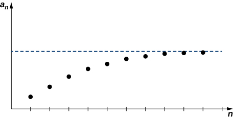
If \(\{a_n\}\) is a bounded sequence and there exists a \(n_0 \in \mathbb{N}\) such that \(\{a_n\}\) is monotone for all \(n \geq n_0\), then \(\{a_n\}\) converges.

The proof of this theorem is beyond the scope of this text. Instead, we provide a graph to show intuitively why this theorem makes sense (Figure \(\PageIndex{6}\)).

Figure \(\PageIndex{6}\): Since the sequence \(\{a_n\}\) is increasing and bounded above, it must converge.

In the following example, we show how the Monotone Convergence Theorem can be used to prove convergence of a sequence.

Example \(\PageIndex{6}\): Using the Monotone Convergence Theorem

For each of the following sequences, use the Monotone Convergence Theorem to show the sequence converges and find its limit.

1. \(\left\{\frac{4^n}{n!}\right\}\)
2. \(\{a_n\}\) defined recursively such that\[a_1=2 \text{ and } a_{n+1}=\dfrac{a_n}{2}+\dfrac{1}{2a_n} \text{ for all } n \geq 2. \nonumber \]

Solution

a. Writing out the first few terms, we see that

\[\left\{\dfrac{4^n}{n!}\right\}=\left\{4,\,8,\,\dfrac{32}{3},\,\dfrac{32}{3},\,\dfrac{128}{15},\, \ldots \right\}.\nonumber \]

At first, the terms increase. However, after the third term, the terms decrease. In fact, the terms decrease for all \(n \geq 3\). We can show this as follows.

\[a_{n+1}=\dfrac{4^{n+1}}{(n+1)!}=\dfrac{4}{n+1} \cdot \dfrac{4^n}{n!}=\dfrac{4}{n+1} \cdot a_n \leq a_n \text{ if } n \geq 3. \nonumber \]

Therefore, the sequence is decreasing for all \(n \geq 3\). Further, the sequence is bounded below by \(0\) because \(4n/n! \geq 0\) for all \( n \in \mathbb{N} \). Therefore, by the Monotone Convergence Theorem, the sequence converges.

To find the limit, we use the fact that the sequence converges and let \(\displaystyle L=\lim_{n \to \infty }a_n\). Now note this important observation. Consider \(\displaystyle \lim_{n \to \infty }a_{n+1}\). Since

\[\{a_{n+1}\}=\{a_2,\,a_3,\,a_4,\, \ldots \},\nonumber \]

the only difference between the sequences \(\{a_{n+1}\}\) and \(\{a_n\}\) is that \(\{a_{n+1}\}\) omits the first term. Since a finite number of terms does not affect the convergence of a sequence,

\[ \lim_{n \to \infty }a_{n+1}=\lim_{n \to \infty }a_n=L. \nonumber \]

Combining this fact with the equation

\[a_{n+1}=\dfrac{4}{n+1}a_n \nonumber \]

and taking the limit of both sides of the equation

\[ \lim_{n \to \infty }a_{n+1}=\lim_{n \to \infty }\dfrac{4}{n+1}a_n, \nonumber \]

we can conclude that

\[L=0 . \nonumber \]

b. Writing out the first several terms,

\[\left\{2,\,\dfrac{5}{4},\,\dfrac{41}{40},\,\dfrac{3281}{3280},\, \ldots \right\}.\nonumber \]

we can conjecture that the sequence is decreasing and bounded below by \(1\). To show that the sequence is bounded below by \(1\), we can show that

\[\dfrac{a_n}{2}+\dfrac{1}{2a_n} \geq 1.\nonumber \]

To show this, first rewrite

\[\dfrac{a_n}{2}+\dfrac{1}{2a_n}=\dfrac{a^2_n+1}{2a_n}. \nonumber \]

Since \(a_1 \gt 0\) and \(a_2\) is defined as a sum of positive terms, \(a_2 \gt 0.\) Similarly, all terms \(a_n \gt 0\). Therefore,

\[\dfrac{a^2n+1}{2a_n} \geq 1 \nonumber \]

if and only if

\[a^2_n+1 \geq 2a_n. \nonumber \]

Rewriting the inequality \(a^2_n+1 \geq 2a_n\) as \(a^2_n−2a_n+1 \geq 0\), and using the fact that

\[a^2_n−2a_n+1=(a_n−1)^2 \geq 0\nonumber \]

because the square of any real number is nonnegative, we can conclude that

\[\dfrac{a^n}{2}+\dfrac{1}{2a_n} \geq 1. \nonumber \]

To show that the sequence is decreasing, we must show that \(a_{n+1} \leq a_n\) for all \(n \geq 1\). Since \(1 \leq a^2_n\), it follows that

\[a^2_n+1 \leq 2a^2_n. \nonumber \]

Dividing both sides by \(2a_n\), we obtain

\[\dfrac{a_n}{2}+\dfrac{1}{2a_n} \leq a_n. \nonumber \]

Using the definition of \(a_{n+1}\), we conclude that

\[a_{n+1}=\dfrac{a_n}{2}+\dfrac{1}{2a_n} \leq a_n. \nonumber \]

Since \(\{a_n\}\) is bounded below and decreasing, by the Monotone Convergence Theorem, it converges.

To find the limit, let \(\displaystyle L=\lim_{n \to \infty }a_n\). Then using the recurrence relation and the fact that \(\displaystyle \lim_{n \to \infty }a_n=\lim_{n \to \infty }a_{n+1}\), we have

\[ \lim_{n \to \infty }a_{n+1}=\lim_{n \to \infty }(\dfrac{a_n}{2}+\dfrac{1}{2a_n}), \nonumber \]

and therefore

\[L=\dfrac{L}{2}+\dfrac{1}{2L}. \nonumber \]

Multiplying both sides of this equation by \(2L\), we arrive at the equation

\[2L^2=L^2+1. \nonumber \]

Solving this equation for \(L,\) we conclude that \(L^2=1\), which implies \(L= \pm 1\). Since all the terms are positive, the limit \(L=1\).

Exercise \(\PageIndex{6}\)

Consider the sequence \(\{a_n\}\) defined recursively such that \(a_1=1\), \(a_n=a_{n−1}/2\). Use the Monotone Convergence Theorem to show that this sequence converges and find its limit.

Hint

Show the sequence is decreasing and bounded below.

Answer

\(0\).

Definition: Fibonacci Numbers

The Fibonacci numbers are defined recursively by the sequence \(\left\{F_n\right\}\) where \(F_0=0\), \(F_1=1\), and for \(n \geq 2\),

\[F_n=F_{n−1}+F_{n−2}. \nonumber \]

Here we look at properties of the Fibonacci numbers.

1. Write out the first twenty Fibonacci numbers.

2. Find a closed formula for the Fibonacci sequence by using the following steps.

a. Consider the recursively defined sequence \({x_n}\) where \(x_0=c\) and \(x_{n+1}=ax_n\). Show that this sequence can be described by the closed formula \(x_n=ca^n\) for all \(n \geq 0\).

b. Using the result from part a. as motivation, look for a solution of the equation

\[F_n=F_{n−1}+F_{n−2} \nonumber \]

of the form \(F_n=c \lambda^n\). Determine what two values for \(\lambda\) will allow \(F_n\) to satisfy this equation.

c. Consider the two solutions from part b.: \(\lambda_1\) and \(\lambda_2\). Let \(F_n=c_1\lambda_1^n+c_2\lambda_2^n\). Use the initial conditions \(F_0\) and \(F_1\) to determine the values for the constants \(c_1\) and \(c_2\) and write the closed formula \(F_n\).

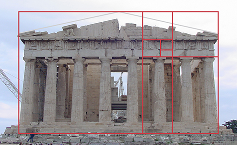
3. Use the answer in 2 c. to show that

\[\lim_{n \to \infty }\dfrac{F_{n+1}}{F_n}=\dfrac{1+\sqrt{5}}{2}.\nonumber \]

The number \(\phi=(1+\sqrt{5})/2\) is known as the golden ratio (Figure \( \PageIndex{7} \) and Figure \( \PageIndex{8} \)).

Figure \(\PageIndex{7}\): The seeds in a sunflower exhibit spiral patterns curving to the left and to the right. The number of spirals in each direction is always a Fibonacci number—always. (credit: modification of work by Esdras Calderan, Wikimedia Commons)

Figure \(\PageIndex{8}\): The proportion of the golden ratio appears in many famous examples of art and architecture. The ancient Greek temple known as the Parthenon was designed with these proportions, and the ratio appears again in many of the smaller details. (credit: modification of work by TravelingOtter, Flickr).

Subsection Footnotes

⁵ When it comes to conditions for something to be true, the words "necessary" and "sufficient" are important in mathematics, and understanding the difference between the two will be helpful.

If a condition is necessary for a result to be true, it means that the necessary condition must exist for the result to even be possible. It does not mean, however, that the existence of the necessary condition immediately implies the result is true. For example, a necessary condition for you to pass this class is that you attend all of the exams; however, just attending the exams is not enough to guarantee you will pass the course.

A sufficient condition, on the other hand, means that, as long as the sufficient condition is met, the result will be true. For example, scoring 80% on all of the exams and assignments in this class is a sufficient condition to passing the class. Note, however, that this is not the only way you can pass this class. For example, earning a 96% on all of the exams and assignments will allow you to pass as well.

The takeaway:

• A sufficient condition guarantees the truth of another condition, but is not necessary for that other condition to happen.
• A necessary condition is required for something else to happen, but it does not guarantee that the something else happens.

Much confusion can be had with necessary and sufficient conditions, but that investigation is left for a course in logic.

---

Key Concepts

• To determine the convergence of a sequence given by an explicit formula \(a_n=f(n)\), we use the properties of limits for functions.
• If \(\{a_n\}\) and \(\{b_n\}\) are convergent sequences that converge to \(A\) and \(B,\) respectively, and \(c\) is any real number, then the sequence \(\{ca_n\} \)converges to \(c\cdot A,\) the sequences \(\{a_n \pm b_n\}\) converge to \(A \pm B,\) the sequence \(\{a_n\cdot b_n\}\) converges to \(A \cdot B,\) and the sequence \(\{a_n/b_n\}\) converges to \(A/B,\) provided \(B \neq 0.\)
• If a sequence is bounded and monotone, then it converges, but not all convergent sequences are monotone.
• If a sequence is unbounded, it diverges, but not all divergent sequences are unbounded.
• The geometric sequence \(\left\{r^n\right\}\) converges if and only if \(|r|<1\) or \(r=1\).

---

Glossary

arithmetic sequence

a sequence in which the difference between every pair of consecutive terms is the same is called an arithmetic sequence

bounded above

a sequence \(\{a_n\}\) is bounded above if there exists a constant \(M\) such that \(a_n \leq M\) for all positive integers \(n\)

bounded below

a sequence \(\{a_n\}\) is bounded below if there exists a constant \(M\) such that \(M \leq a_n\) for all positive integers \(n\)

bounded sequence

a sequence \(\{a_n\}\) is bounded if there exists a constant \(M\) such that \(|a_n| \leq M\) for all positive integers \(n\)

convergent sequence

a convergent sequence is a sequence \(\{a_n\}\) for which there exists a real number \(L\) such that \(a_n\) is arbitrarily close to \(L\) as long as \(n\) is sufficiently large

divergent sequence

a sequence that is not convergent is divergent

explicit formula

a sequence may be defined by an explicit formula such that \(a_n=f(n)\)

geometric sequence

a sequence \(\{a_n\}\) in which the ratio \(a_{n+1}/a_n\) is the same for all positive integers \(n\) is called a geometric sequence

index variable

the subscript used to define the terms in a sequence is called the index

limit of a sequence

the real number \(L\) to which a sequence converges is called the limit of the sequence

monotone sequence

an increasing or decreasing sequence

recurrence relation

a recurrence relation is a relationship in which a term \(a_n\) in a sequence is defined in terms of earlier terms in the sequence

sequence

an ordered list of numbers of the form \(a_1,\,a_2,\,a_3,\, \ldots \) is a sequence

term

the number \(a_n\) in the sequence \(\{a_n\}\) is called the \(n^{\text{th}}\) term of the sequence

unbounded sequence

a sequence that is not bounded is called unbounded