3.9: Inverse Functions
( \newcommand{\kernel}{\mathrm{null}\,}\)
- Determine if a function is 1-1.
- Determine the domain and range of an inverse function, and restrict the domain of a function to make it one-to-one.
- Find or evaluate the inverse of a function.
- Verify inverse functions.
- Use the graph of a one-to-one function to graph its inverse function on the same axes.
Try these questions prior to beginning this section to help determine if you are set up for success:
- Simplify: 2+1x1x−8
- What is the domain of f(x)=√2x−5. State your answer in interval notation.
- Answer
-
- 2x+11−8x, If you missed this problem or feel you could use more practice, review [2.14: Adding and Subtracting Rational Expressions]
- [52,∞), If you missed this problem or feel you could use more practice, review [3.3: Functions and Function Notation]
A reversible heat pump is a climate-control system that is an air conditioner and a heater in a single device. Operated in one direction, it pumps heat out of a house to provide cooling. Operating in reverse, it pumps heat into the building from the outside, even in cool weather, to provide heating. As a heater, a heat pump is several times more efficient than conventional electrical resistance heating.
If some physical machines can run in two directions, we might ask whether some of the function “machines” we have been studying can also run backwards. Figure 3.9.1 provides a visual representation of this question. In this section, we will consider the reverse nature of functions.
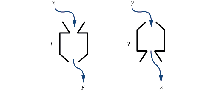
Figure 3.9.1: Can a function “machine” operate in reverse?
This idea of operating a function in reverse is known as an inverse operation. It is important when doing so that we know if the inverse is itself a function also. Let's take a moment to review what a function is and how we may determine if an inverse of a function will itself be a function.
Recall: A function of (\x\) is a relation in which each input, (\x\), value in the domain is assigned to exactly one output, value in the range.
One-to-One Functions
Some functions have a given output value that corresponds to two or more input values. However, some functions have only one input value for each output value, as well as having only one output for each input. We call these functions one-to-one functions.
To visualize this concept, let’s look again at some simple relations in Figures 3.9.2 below. The function in part (a) shows a relationship that is not a one-to-one function because inputs q and r both give output n. The function in part (b) shows a relationship that is a one-to-one function because each input is associated with a single output.
![[Three relations that demonstrate what constitute a function.]](https://math.libretexts.org/@api/deki/files/861/CNX_Precalc_Figure_01_01_001.jpg?revision=1)
A one-to-one function is a function in which each output value corresponds to exactly one input value.
Is the area of a circle a function of its radius? If yes, is the function one-to-one?
Solution
A circle of radius r has a unique area measure given by A=πr2, so for any input, r, there is only one output, A. The area is a function of radiusr.
If the function is one-to-one, the output value, the area, must correspond to a unique input value, the radius. Any area measure A is given by the formula A=πr2. Because areas and radii are positive numbers, there is exactly one solution:√Aπ. So the area of a circle is a one-to-one function of the circle’s radius.
- Is a balance in a bank account a function of the bank account number?
- Is a bank account number a function of the balance?
- Is a balance a one-to-one function of the bank account number?
- Answer
-
- yes, because each bank account has a single balance at any given time;
- no, because several bank account numbers may have the same balance;
- no, because the same output may correspond to more than one input.
Horizontal Line Test
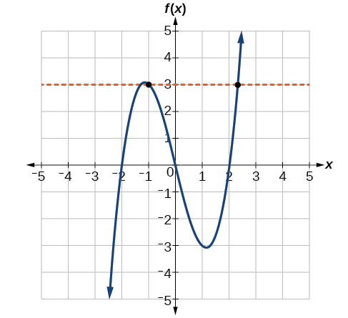
An easy way to determine if a function is a one-to-one function is to use the horizontal line test. Draw horizontal lines through the graph. If any horizontal line intersects the graph more than once, as seen in Figure 3.9.3, then the graph does not represent a one-to-one function.
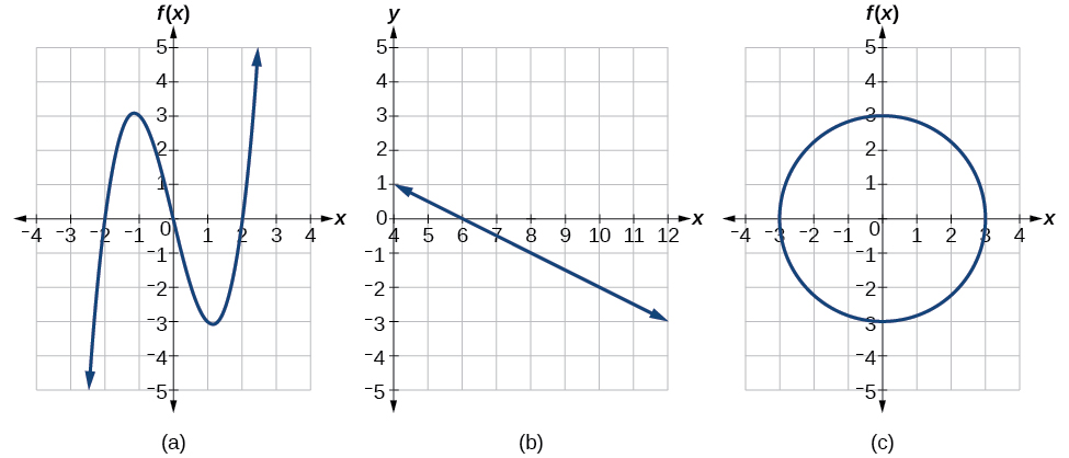
Consider the relations shown below in Figure 3.9.4. Are any of these one-to-one functions?
Solution
The graphs in (a) and (b) are functions since they satisfy the vertical line test. The graph in (a) is not a one-to-one function since a horizontal line will intersect the graph more than once. The graph in (b) is a one-to-one function since there is not any horizontal line that will intersect the graph more than once. The graph is part (c) is not a function so it not a one-to-one function.
Inverse Functions
Suppose a fashion designer will be traveling to Milan for a fashion show and wants to know what the temperature will be. She finds the weather forecast online, as shown in Figure 3.9.5. She is not familiar with the Celsius scale and her internet connection went down right after she found the forecast. She decided to convert the temperature from degrees Celsius to degrees Fahrenheit because she remembers the formula
C=59(F−32)
75 degrees Fahrenheit is a comfortable temperature for his. So, she substitutes 75 for F into the formula
59(75−32)≈24∘
and finds that 75 degrees Fahrenheit is about 24 degrees Celsius.

She could do this for other temperatures but quickly realized that the most efficient thing to do is solve the equation for F. Then she can just plug in the Celsius degrees into the equation and evaluate to get the temperatures in Fahrenheit degrees. The equation, F=95C+32 is known as an inverse function.
If f(x)=y, then a function g is an inverse of f if g(y)=x.
The inverse function of f(x) is typically notated as f−1(x), which is read “f inverse of x”. , so equivalently, if f(x)=y then f−1(y)=x.
The notation f−1(x) may only be used when the inverse of f is itself a a function. There are some functions that do not have inverse functions.
The -1 used in the notation f−1(x) is simply a function notation where the name of the function is "f inverse", and does not designate an exponent or power of -1.
Keep in mind that f−1(x)≠1f(x)
Given that h−1(6)=2, what are the corresponding input and output values of the original function h?
Solution
h(2)=6
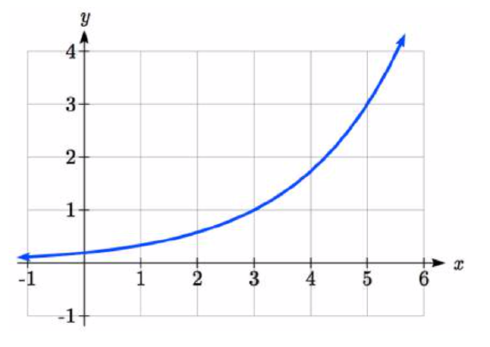
A function g(x) is given as a graph below. Find g(3) and g−1(3)
Solution
To evaluate g(3), we find 3 on the horizontal axis and find the corresponding output value on the vertical axis. The point (3, 1) tells us that g(3)=1
To evaluate g−1(3), recall that by definition g−1(3) means g(x)=3. By looking for the output value 3 on the vertical axis we find the point (5, 3) on the graph, which means g(5)=3, so by definition g−1(3)=5.
A function f(t) is given as a table below, showing distance in miles that a car has traveled in t minutes. Find and interpret f−1(70)
| t (minutes) | 30 | 50 | 70 | 90 |
| f(t) (miles) | 20 | 40 | 60 | 70 |
Solution
The inverse function takes an output of f and returns an input for f. So in the expression f−1(70), the 70 is an output value of the original function, representing 70 miles. The inverse will return the corresponding input of the original function f, 90 minutes, so f−1(70)=90. Interpreting this, it means that to drive 70 miles, it took 90 minutes.
Alternatively, recall the definition of the inverse was that if f(a)=b then f−1(b)=a. By this definition, if you are given f−1(70)=a then you are looking for a value a so that f(a)=70. In this case, we are looking for a t so that f(t)=70, which is when t=90.
Notice that original function and the inverse function undo each other. If f(a)=b, then f−1(b)=a, returning us to the original input. More simply put, if you compose a function and its inverse function together, you get the original input as your answer. Composition may be used to verify this.
Determining if Two Functions are Inverses of Each Other
For two one-to-one functions, f and g,
- Determine whether f(g(x))=x and g(f(x))=x.
- If both statements in part (1) are true, then the functions are inverses of each other (g=f−1 and f=g−1). If one or both statements in part (1) are false, then the functions are not inverses of each other (g≠f−1 and f≠g−1).
If f(x)=1x+2 and g(x)=1x−2, is g=f−1?
Solution
g(f(x))=1(1x+2)−2=x+2−2=x
so
g=f−1 and f=g−1
This is enough to answer yes to the question, but we can also verify the other formula.
f(g(x))=1(1x−2)+2=11x=x
If f(x)=x3−4 and g(x)=3√x+4, is g=f−1?
- Answer
-
Yes
If f(x)=x3 (the basic cubic function) and g(x)=13x, is g=f−1?
Solution
f(g(x))=x327≠x
No, the functions are not inverses.
Note that the correct inverse to the basic cubic function is, of course, the cube root 3√x=x13, that is, the one-third is an exponent, not a multiplier.
If f(x)=(x−1)3 and g(x)=3√x+1, is g=f−1?
- Answer
-
Yes
Domain and Range of Inverse Functions
We have seen that the outputs of the function f are the inputs to f−1, so the range of f is also the domain of f−1. Likewise, because the inputs to f are the outputs of f−1, the domain of f is the range of f−1. We can visualize the situation as in Figure 3.9.6.

Figure 3.9.6: Domain and range of a function and its inverse.
This is important to remember when finding inverse functions. For example, the inverse of f(x)=√x is f−1(x)=x2,x≥0, because a square “undoes” a square root; but the square is only the inverse of the square root on the domain [0,∞), since that is the range of f(x)=√x.
Finding Inverses of Functions Represented by Formulas
Sometimes we will need to know an inverse function for all elements of its domain, not just a few. If the original function is given as a formula— for example, y as a function of x— we can often find the inverse function by solving to obtain x as a function of y.
- Make sure f is a one-to-one function.
- Solve for x
- Interchange x and y to write the inverse as a function of x. Do remember to include any restrictions for the domain if it is not clearly implied in the equation you found.
Returning to our designer traveling to Milan, find a formula for the inverse function that gives Fahrenheit temperature given a Celsius temperature.
Solution
A quick Google search would find the inverse function, but alternatively, the designer might look back at how she solved for the Fahrenheit temperature for a specific Celsius value, and repeat the process in general
C=59(F−32)C⋅95=F−32F=95C+32
By solving in general, we have uncovered the inverse function. If
C=h(F)=59(F−32)
Then
F=h−1(C)=95C+32
In this case, we introduced a notation for a function h to represent the conversion since the input and output variables are descriptive and writing C−1 could get confusing.
Find the inverse of the function f(x)=2+√x−4.
Solution
y=2+√x−4y−2=√x−4(y−2)2=x−4x=(y−2)2+4
interchanging x and y,
y=(x−2)2+4
Notice that the range of f is [2,∞), so this means that the domain of the inverse function f−1 is also [2,∞). The formula we found for f−1(x) above looks like it would be valid for all real x. However, f−1 itself must have an inverse (namely, f ) so we have to state the restricted domain of f−1 to [2,∞) in order to make f−1 a one-to-one function.
So, f−1(x)=(x−2)2+4 where x≥2.
What is the inverse of the function f(x)=2−√x?
- Answer
-
f−1(x)=(2−x)2 where x≤2
Inverse Functions and Their Graphs
Now that we know how to find the inverse of a function, let's explore the graphical relationship of functions and their inverses. Let's look at the quadratic function f(x)=x2 restricted to the domain [0,∞). This is a one-to-one function, and it's graph is shown in Figure 3.9.7.
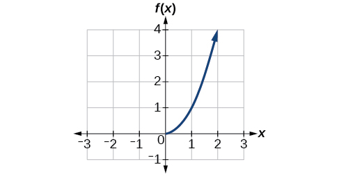
Figure 3.9.7: Quadratic function with domain restricted to [0,∞).
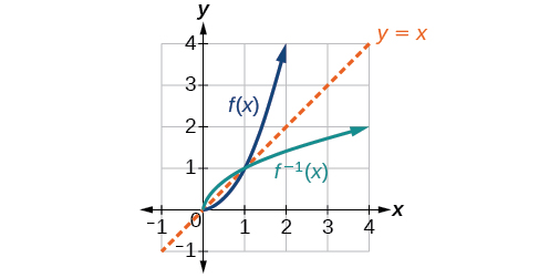
The inverse of this function is f−1(x)=√x. The graph of both f and f−1 are shown in Figure 3.9.8 on the same set of axes.
Notice that the graph of f−1(x) is the graph of f(x) reflected about the diagonal line y=x, which we will call the identity line, shown in Figure 3.9.8.
 .
.
Figure 3.9.8: Square and square-root functions on the non-negative domain
This relationship will be observed for all one-to-one functions and their inverses, because it is a result of the function and its inverse swapping inputs and outputs. This is useful to know for checking for errors when finding an inverse of a one-to-one function since the inverse equation found should visually be a reflection over the line (y=x\).
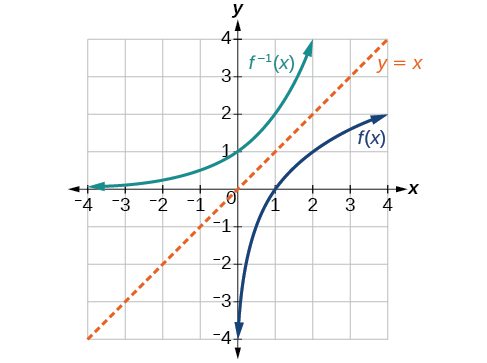
Given the graph of f(x) in Figure 3.9.9, sketch a graph of f−1(x).
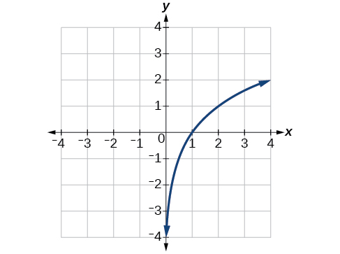
This is a one-to-one function, so we will be able to sketch an inverse. Note that the graph shown has an apparent domain of (0,∞) and range of (−∞,∞), so the inverse will have a domain of (−∞,∞) and range of (0,∞).
If we reflect this graph over the line y=x, the point (1,0) reflects to (0,1), the point (4,2) reflects to (2,4), and so on. Sketching the inverse on the same axes as the original graph gives Figure 3.9.10.
![]() Is there any function that is equal to its own inverse?
Is there any function that is equal to its own inverse?
Yes. If f=f−1, then f(f(x))=x, and we can think of several functions that have this property. The identity function
does, and so does the basic reciprocal function, because
11x=x
Any function f(x)=c−x, where c is a constant, is also equal to its own inverse.
Contributors and Attributions
Jay Abramson (Arizona State University) with contributing authors. Textbook content produced by OpenStax College is licensed under a Creative Commons Attribution License 4.0 license. Download for free at https://openstax.org/details/books/precalculus.


