4.7: Quadratic Functions

You may recall studying quadratic equations in Intermediate Algebra. In this section, we review those equations in the context of our next family of functions: the quadratic functions.

definition 2.5: quadratic function

A quadratic function is a function of the form

$$f(x) = ax^2 + bx + c, \label{quadraticfunction}$$

where $a$, $b$ and $c$ are real numbers with $a \neq 0$. The domain of a quadratic function is $(-\infty, \infty)$.

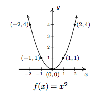
The most basic quadratic function is $f(x) = x^2$, whose graph appears below. Its shape should look familiar from Intermediate Algebra -- it is called a parabola. The point $(0,0)$ is called the vertex of the parabola. In this case, the vertex is a relative minimum and is also the where the absolute minimum value of $f$ can be found.

Much like many of the absolute value functions in Section 2.2, knowing the graph of $f(x) = x^2$ enables us to graph an entire family of quadratic functions using transformations.

Example $\PageIndex{1}$:

Graph the following functions starting with the graph of $f(x) = x^2$ and using transformations. Find the vertex, state the range and find the $x$- and $y$-intercepts, if any exist.

1. $g(x) = (x+2)^2 - 3$
2. $h(x) = -2(x-3)^2+1$

Solution

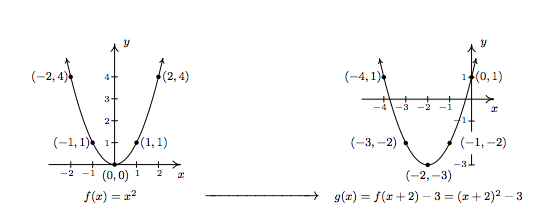
1. Since $g(x) = (x+2)^2 - 3 = f(x+2) - 3$, Theorem 1.7 instructs us to first $\textit{subtract}$ $2$ from each of the $x$-values of the points on $y=f(x)$. This shifts the graph of $y = f(x)$ to the $\textit{left}$ $2$ units and moves $(-2,4)$ to $(-4,4)$, $(-1,1)$ to $(-3,1)$, $(0,0)$ to $(-2,0)$, $(1,1)$ to $(-1,1)$ and $(2,4)$ to $(0,4)$. Next, we $\textit{subtract}$ $3$ from each of the $y$-values of these new points. This moves the graph $\textit{down}$ $3$ units and moves $(-4,4)$ to $(-4,1)$, $(-3,1)$ to $(-3,-2)$, $(-2,0)$ to $(-2,3)$, $(-1,1)$ to $(-1,-2)$ and $(0,4)$ to $(0,1)$. We connect the dots in parabolic fashion to get

From the graph, we see that the vertex has moved from $(0,0)$ on the graph of $y = f(x)$ to $(-2,-3)$ on the graph of $y = g(x)$. This sets $[-3, \infty)$ as the range of $g$. We see that the graph of $y=g(x)$ crosses the $x$-axis twice, so we expect two $x$-intercepts. To find these, we set $y = g(x) = 0$ and solve. Doing so yields the equation $(x+2)^2 - 3 = 0$, or $(x+2)^2 = 3$. Extracting square roots gives $x + 2 = \pm \sqrt{3}$, or $x = -2 \pm \sqrt{3}$. Our $x$-intercepts are $(-2-\sqrt{3}, 0) \approx (-3.73, 0)$ and $(-2+\sqrt{3}, 0) \approx (-0.27, 0)$. The $y$-intercept of the graph, $(0,1)$ was one of the points we originally plotted, so we are done.

2. Following Theorem 1.7 once more, to graph $h(x) = -2(x-3)^2+1 = -2f(x-3)+1$, we first start by $\textit{adding}$ $3$ to each of the $x$-values of the points on the graph of $y=f(x)$. This effects a horizontal shift $\textit{right}$ $3$ units and moves $(-2,4)$ to $(1,4)$, $(-1,1)$ to $(2,1)$, $(0,0)$ to $(3,0)$, $(1,1)$ to $(4,1)$ and $(2,4)$ to $(5,4)$. Next, we $\textit{multiply}$ each of our $y$-values first by $-2$ and then $\textit{add}$ $1$ to that result. Geometrically, this is a vertical $\textit{stretch}$ by a factor of $2$, followed by a reflection about the $x$-axis, followed by a vertical shift $\textit{up}$ $1$ unit. This moves $(1,4)$ to $(1,-7)$, $(2,1)$ to $(2,-1)$, $(3,0)$ to $(3,1)$, $(4,1)$ to $(4,-1)$ and $(5,4)$ to $(5,-7)$.

The vertex is $(3,1)$ which makes the range of $h$ $(-\infty, 1]$. From our graph, we know that there are two $x$-intercepts, so we set $y = h(x) = 0$ and solve. We get $-2(x-3)^2+1 = 0$ which gives $(x-3)^2 = \frac{1}{2}$. Extracting square roots\footnote{and rationalizing denominators!} gives $x - 3 = \pm \frac{\sqrt{2}}{2}$, so that when we add $3$ to each side,\footnote{and get common denominators!} we get $x = \frac{6 \pm \sqrt{2}}{2}$. Hence, our $x$-intercepts are $\left(\frac{6 - \sqrt{2}}{2}, 0 \right) \approx (2.29, 0)$ and $\left(\frac{6 + \sqrt{2}}{2}, 0 \right) \approx (3.71, 0)$. Although our graph doesn't show it, there is a $y$-intercept which can be found by setting $x=0$. With $h(0) = -2(0-3)^2+1 = -17$, we have that our $y$-intercept is $(0,-17)$. $\Box$

A few remarks about Example $\PageIndex{1}$ are in order. First note that neither the formula given for $g(x)$ nor the one given for $h(x)$ match the form given in Definition 2.5. We could, of course, convert both $g(x)$ and $h(x)$ into that form by expanding and collecting like terms. Doing so, we find $g(x) = (x+2)^2 - 3 = x^2 + 4x+1$ and $h(x) = -2(x-3)^2+1 = -2x^2+12x-17$. While these `simplified' formulas for $g(x)$ and $h(x)$ satisfy Definition 2.5, they do not lend themselves to graphing easily. For that reason, the form of $g$ and $h$ presented in Example $\PageIndex{2}$ is given a special name, which we list below, along with the form presented in Definition 2.5.

Definition 2.6: Standard and General Form of Quadratic Functions

Suppose $f$ is a quadratic function.

• The general form of the quadratic function $f$ is $$f(x) = ax^2+bx+c$$ where $a$, $b$ and $c$ are real numbers with $a \neq 0$.
• The standard form of the quadratic function $f$ is $$f(x) = a(x-h)^2 + k$$ where $a$, $h$ and $k$ are real numbers with $a\neq 0$.

It is important to note at this stage that we have no guarantees that $\textit{every}$ quadratic function can be written in standard form. This is actually true, and we prove this later in the exposition, but for now we celebrate the advantages of the standard form, starting with the following theorem.

Theorem 2.2: Vertex Formula for Quadratics in Standard Form

For the quadratic function $f(x) = a(x-h)^2 + k$, where $a$, $h$ and $k$ are real numbers with $a\neq 0$, the vertex of the graph of $y = f(x)$ is $(h,k)$.

We can readily verify the formula given Theorem 2.2 with the two functions given in Example $\PageIndex{1}$. After a (slight) rewrite, $g(x) = (x+2)^2 - 3 = (x-(-2))^2+(-3)$, and we identify $h=-2$ and $k=-3$. Sure enough, we found the vertex of the graph of $y=g(x)$ to be $(-2,-3)$. For $h(x) = -2(x-3)+1$, no rewrite is needed. We can directly identify $h=3$ and $k=1$ and, sure enough, we found the vertex of the graph of $y=h(x)$ to be $(3,1)$.

To see why the formula in Theorem 2.2 produces the vertex, consider the graph of the equation $y = a(x-h)^2 + k$. When we substitute $x=h$, we get $y=k$, so $(h,k)$ is on the graph. If $x \neq h$, then $x-h \neq 0$ so $(x-h)^2$ is a positive number. If $a>0$, then $a(x-h)^2$ is positive, thus $y = a(x-h)^2 + k$ is always a number larger than $k$. This means that when $a>0$, $(h,k)$ is the lowest point on the graph and thus the parabola must open upwards, making $(h,k)$ the vertex. A similar argument shows that if $a<0$, $(h,k)$ is the highest point on the graph, so the parabola opens downwards, and $(h,k)$ is also the vertex in this case.

Alternatively, we can apply the machinery in Section 1.7. Since the vertex of $y = x^2$ is $(0,0)$, we can determine the vertex of $y = a(x-h)^2+k$ by determining the final destination of $(0,0)$ as it is moved through each transformation. To obtain the formula $f(x)= a(x-h)^2+k$, we start with $g(x)=x^2$ and first define $g_1(x) = a g(x) = ax^2$. This is results in a vertical scaling and/or reflection.\footnote{Just a scaling if $a>0$. If $a<0$, there is a reflection involved.} Since we multiply the output by $a$, we multiply the $y$-coordinates on the graph of $g$ by $a$, so the point $(0,0)$ remains $(0,0)$ and remains the vertex. Next, we define $g_{\mbox{\tiny\(2\)}}(x) = g_{\mbox{\tiny\)1\)}}(x-h) = a(x-h)^2$. This induces a horizontal shift right or left $h$ units\footnote{Right if $h>0$, left if $h<0$.} moves the vertex, in either case, to $(h,0)$. Finally, $f(x) = g_2(x)+k = a(x-h)^2+k$ which effects a vertical shift up or down $k$ units\footnote{Up if $k>0$, down if $k<0$} resulting in the vertex moving from $(h,0)$ to $(h,k)$.

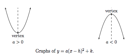
In addition to verifying Theorem 2.2, the arguments in the two preceding paragraphs have also shown us the role of the number $a$ in the graphs of quadratic functions. The graph of $y = a(x-h)^2 + k$ is a parabola `opening upwards' if $a > 0$, and `opening downwards' if $a < 0$. Moreover, the symmetry enjoyed by the graph of $y = x^2$ about the $y$-axis is translated to a symmetry about the vertical line $x=h$ which is the vertical line through the vertex.\footnote{You should use transformations to verify this!} This line is called the $\textbf{axis of symmetry}$ of the parabola and is dashed in the figures below.

Without a doubt, the standard form of a quadratic function, coupled with the machinery in Section 1.7, allows us to list the attributes of the graphs of such functions quickly and elegantly. What remains to be shown, however, is the fact that every quadratic function $\textit{can be written}$ in standard form. To convert a quadratic function given in general form into standard form, we employ the ancient rite of `Completing the Square'. We remind the reader how this is done in our next example.

Example $\PageIndex{2}$:

Convert the functions below from general form to standard form. Find the vertex, axis of symmetry and any $x$- or $y$-intercepts. Graph each function and determine its range.

1. $f(x) = x^2-4x+3$.
2. $g(x) = 6-x-x^2$

Solution

1. To convert from general form to standard form, we complete the square.\footnote{If you forget why we do what we do to complete the square, start with $a(x-h)^2 + k$, multiply it out, step by step, and then reverse the process.} First, we verify that the coefficient of $x^2$ is $1$. Next, we find the coefficient of $x$, in this case $-4$, and take half of it to get $\frac{1}{2}(-4) = -2$. This tells us that our target perfect square quantity is $(x-2)^2$. To get an expression equivalent to $(x-2)^2$, we need to add $(-2)^2 = 4$ to the $x^2-4x$ to create a perfect square trinomial, but to keep the balance, we must also subtract it. We collect the terms which create the perfect square and gather the remaining constant terms. Putting it all together, we get

$$\begin{array}{rclr} f(x) & = & x^2-4x+3 & \text{(Compute \(\frac{1}{2} (-4) = -2\).)} \\ & = & \left(x^2 - 4x + \underline{4} - \underline{4}\right) + 3 & \text{(Add and subtract \((-2)^2 = 4\) to \((x^2+4x)\).)}\\ & = & \left(x^2 - 4x + 4\right) - 4 + 3 & \text{(Group the perfect square trinomial.)}\\ & = & (x-2)^2 - 1 & \text{(Factor the perfect square trinomial.)} \\ \end{array}$$

Of course, we can always check our answer by multiplying out $f(x) = (x-2)^2 -1$ to see that it simplifies to $f(x) = x^2 - 4x - 1$. In the form $f(x) = (x-2)^2-1$, we readily find the vertex to be $(2,-1)$ which makes the axis of symmetry $x = 2$. To find the $x$-intercepts, we set $y = f(x) = 0$. We are spoiled for choice, since we have $\textit{two}$ formulas for $f(x)$. Since we recognize $f(x) = x^2-4x+3$ to be easily factorable,\footnote{Experience pays off, here!} we proceed to solve $x^2-4x+3 = 0$. Factoring gives $(x-3)(x-1) = 0$ so that $x = 3$ or $x=1$. The $x$-intercepts are then $(1,0)$ and $(3,0)$. To find the $y$-intercept, we set $x=0$. Once again, the general form $f(x) = x^2-4x+3$ is easiest to work with here, and we find $y = f(0) = 3$. Hence, the $y$-intercept is $(0,3)$. With the vertex, axis of symmetry and the intercepts, we get a pretty good graph without the need to plot additional points. We see that the range of $f$ is $[-1,\infty)$ and we are done.

2. To get started, we rewrite $g(x) = 6-x-x^2 = -x^2-x+6$ and note that the coefficient of $x^2$ is $-1$, not $1$. This means our first step is to factor out the $(-1)$ from both the $x^2$ and $x$ terms. We then follow the completing the square recipe as above.

$$\begin{array}{rclr} g(x) & = & -x^2-x+6 & \\ & = & (-1)\left(x^2 + x \right) + 6 & \text{(Factor the coefficient of \(x^2\) from \(x^2\) and \(x\).)} \\ & = & (-1)\left(x^2 + x + \underline{\frac{1}{4}} - \underline{\frac{1}{4}} \right) + 6 & \\ & = & (-1)\left(x^2 + x + \frac{1}{4}\right) + (-1)\left(-\frac{1}{4}\right) + 6 & \text{(Group the perfect square trinomial.)}\\ & = & -\left(x +\frac{1}{2}\right)^2 + \frac{25}{4} & \\ \end{array}$$

From $g(x) = -\left(x +\frac{1}{2}\right)^2 + \frac{25}{4}$, we get the vertex to be $\left(-\frac{1}{2}, \frac{25}{4}\right)$ and the axis of symmetry to be $x = -\frac{1}{2}$. To get the $x$-intercepts, we opt to set the given formula $g(x) = 6-x-x^2 = 0$. Solving, we get $x = -3$ and $x=2$, so the $x$-intercepts are $(-3,0)$ and $(2,0)$. Setting $x=0$, we find $g(0) = 6$, so the $y$-intercept is $(0,6)$. Plotting these points gives us the graph below. We see that the range of $g$ is $\left(-\infty, \frac{25}{4}\right]$.

With Example $\PageIndex{2}$ fresh in our minds, we are now in a position to show that every quadratic function can be written in standard form. We begin with $f(x) = ax^2+bx+c$, assume $a \neq 0$, and complete the square in $\textit{complete}$ generality.

$$\begin{array}{rclr} f(x) & = & ax^2 + bx + c & \\ & = & a\left(x^2 + \dfrac{b}{a} x\right) + c & \text{(Factor out coefficient of \(x^2\) from \(x^2\) and \(x\).)} \\ & = & a\left(x^2 + \dfrac{b}{a} x + \underline{\dfrac{b^{2}}{4a^2}} - \underline{\dfrac{b^{2}}{4a^2}} \right) + c & \\ & = & a\left(x^2 + \dfrac{b}{a} x + \dfrac{b^{2}}{4a^2} \right) - a \left(\dfrac{b^{2}}{4a^2}\right) + c & \text{(Group the perfect square trinomial.)} \\ & = & a\left(x+\dfrac{b}{2a}\right)^2 + \dfrac{4ac - b^2}{4a} & \text{(Factor and get a common denominator.)} \\ \end{array}$$

Comparing this last expression with the standard form, we identify $(x-h)$ with $\left(x+\frac{b}{2a}\right)$ so that $h = -\frac{b}{2a}$. Instead of memorizing the value $k = \frac{4ac - b^2}{4a}$, we see that $f\left(-\frac{b}{2a}\right) = \frac{4ac - b^2}{4a}$. As such, we have derived a vertex formula for the general form. We summarize both vertex formulas in the box at the top of the next page.

Equation 2.4: Vertex Formulas for Quadratic Functions

Suppose $a$, $b$, $c$, $h$ and $k$ are real numbers with $a \neq 0$.

• If $f(x) = a(x-h)^2 + k$, the vertex of the graph of $y=f(x)$ is the point $(h,k)$.
• If $f(x) = ax^2+bx+c$, the vertex of the graph of $y=f(x)$ is the point $\left(-\dfrac{b}{2a}, f\left(-\dfrac{b}{2a}\right)\right)$.

There are two more results which can be gleaned from the completed-square form of the general form of a quadratic function,

$$f(x) = ax^2 + bx + c = a\left(x+\dfrac{b}{2a}\right)^2 + \dfrac{4ac - b^2}{4a}$$

We have seen that the number $a$ in the standard form of a quadratic function determines whether the parabola opens upwards (if $a>0$) or downwards (if $a < 0$). We see here that this number $a$ is none other than the coefficient of $x^2$ in the general form of the quadratic function. In other words, it is the coefficient of $x^2$ alone which determines this behavior -- a result that is generalized in Section 3.1. The second treasure is a re-discovery of the quadratic formula.

Equation 2.5: The Quadratic Formula

If $a$, $b$ and $c$ are real numbers with $a \neq 0$, then the solutions to $ax^2 + bx + c = 0$ are

$$x = \dfrac{-b \pm \sqrt{b^2-4ac}}{2a}.\label{equation2.5}$$

Assuming the conditions of Equation 2.5, the solutions to $ax^2+bx+c = 0$ are precisely the zeros of $f(x) = ax^2 + bx + c$. Since

$$f(x) = ax^2+bx+c = a\left(x+\dfrac{b}{2a}\right)^2 + \dfrac{4ac - b^2}{4a}$$

the equation $ax^2 + bx + c = 0$ is equivalent to

$$a\left(x+\dfrac{b}{2a}\right)^2 + \dfrac{4ac - b^2}{4a} = 0.$$

Solving gives

$$\begin{array}{rclr} a\left(x+\dfrac{b}{2a}\right)^2 + \dfrac{4ac - b^2}{4a} & = & 0 & \\ [15pt] a\left(x+\dfrac{b}{2a}\right)^2 & = & - \dfrac{4ac - b^2}{4a} & \\ [15pt] \dfrac{1}{a} \left[a\left(x+\dfrac{b}{2a}\right)^2\right] & = & \dfrac{1}{a} \left(\dfrac{b^2-4ac}{4a}\right) & \\ [15pt] \left(x+\dfrac{b}{2a}\right)^2 & = & \dfrac{b^2-4ac}{4a^2} & \\ [15pt] x+\dfrac{b}{2a} & = & \pm \sqrt{\dfrac{b^2-4ac}{4a^2}} & \mbox{extract square roots} \\ [15pt] x+\dfrac{b}{2a} & = & \pm \dfrac{\sqrt{b^2-4ac}}{2a} & \\ [15pt] x & = & -\dfrac{b}{2a} \pm \dfrac{\sqrt{b^2-4ac}}{2a} \\ [15pt] x & = & \dfrac{-b \pm \sqrt{b^2-4ac}}{2a} & \end{array}$$

In our discussions of domain, we were warned against having negative numbers underneath the square root. Given that $\sqrt{b^{2} - 4ac}$ is part of the Quadratic Formula, we will need to pay special attention to the radicand $b^{2} - 4ac$. It turns out that the quantity $b^2-4ac$ plays a critical role in determining the nature of the solutions to a quadratic equation. It is given a special name.

Definition 2.7: discriminant

If $a$, $b$ and $c$ are real numbers with $a \neq 0$, then the discriminant of the quadratic equation $ax^2+bx+c=0$ is the quantity

$$b^2 - 4ac.\label{discriminant}$$

The discriminant `discriminates' between the kinds of solutions we get from a quadratic equation. These cases, and their relation to the discriminant, are summarized below.

Theorem 2.3: Discriminant Trichotomy

Let $a$, $b$ and $c$ be real numbers with $a \neq 0$.

• If $b^2 - 4ac < 0$, the equation $ax^2 + bx + c = 0$ has no real solutions.
• If $b^2 - 4ac = 0$, the equation $ax^2 + bx + c = 0$ has exactly one real solution.
• If $b^2 - 4ac > 0$, the equation $ax^2 + bx + c = 0$ has exactly two real solutions.

The proof of Theorem 2.3 stems from the position of the discriminant in the quadratic equation, and is left as a good mental exercise for the reader. The next example exploits the fruits of all of our labor in this section thus far.

Example $\PageIndex{3}$:

Recall that the profit (Section 1.4) for a product is defined by the equation $\mbox{Profit} = \mbox{Revenue} - \mbox{Cost}$, or $P(x) = R(x) - C(x)$. In Example 2.1.7 the weekly revenue, in dollars, made by selling $x$ PortaBoy Game Systems was found to be $R(x) = -1.5x^2+250x$ with the restriction (carried over from the price-demand function) that $0 \leq x \leq 166$. The cost, in dollars, to produce $x$ PortaBoy Game Systems is given in Example 2.1.5 as $C(x) = 80x + 150$ for $x \geq 0$.

1. Determine the weekly profit function $P(x)$.
2. Graph $y = P(x)$. Include the $x$- and $y$-intercepts as well as the vertex and axis of symmetry.
3. Interpret the zeros of $P$.
4. Interpret the vertex of the graph of $y = P(x)$.
5. Recall that the weekly price-demand equation for PortaBoys is $p(x) = -1.5x+250$, where $p(x)$ is the price per PortaBoy, in dollars, and $x$ is the weekly sales. What should the price per system be in order to maximize profit?

Solution

1. To find the profit function $P(x)$, we subtract $$P(x) = R(x) - C(x) = \left(-1.5x^2+250x\right) - \left(80x + 150\right) = -1.5x^2+170x-150.$$ Since the revenue function is valid when $0 \leq x \leq 166$, $P$ is also restricted to these values.
2. To find the $x$-intercepts, we set $P(x) = 0$ and solve $-1.5x^2+170x-150=0$. The mere thought of trying to factor the left hand side of this equation could do serious psychological damage, so we resort to the quadratic formula, Equation 2.5. Identifying $a = -1.5$, $b=170$, and $c=-150$, we obtain

$$\begin{array}{rclr} x & = & \dfrac{-b \pm \sqrt{b^2-4ac}}{2a} & \\ & = & \dfrac{-170 \pm \sqrt{170^2 - 4(-1.5)(-150)}}{2(-1.5)} & \\ & = & \dfrac{-170 \pm \sqrt{28000}}{-3} & \\ & = & \dfrac{170 \pm 20 \sqrt{70}}{3} & \\ \end{array}$$

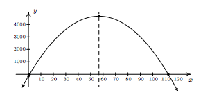
We get two $x$-intercepts: $\left( \frac{170 - 20 \sqrt{70}}{3},0\right)$ and $\left( \frac{170 + 20 \sqrt{70}}{3},0\right)$. To find the $y$-intercept, we set $x=0$ and find $y=P(0)=-150$ for a $y$-intercept of $(0,-150)$. To find the vertex, we use the fact that $P(x)=-1.5x^2+170x-150$ is in the general form of a quadratic function and appeal to Equation 2.4. Substituting $a = -1.5$ and $b=170$, we get $x = -\frac{170}{2(-1.5)} = \frac{170}{3}$. To find the $y$-coordinate of the vertex, we compute $P\left( \frac{170}{3} \right) = \frac{14000}{3}$ and find that our vertex is $\left(\frac{170}{3}, \frac{14000}{3}\right)$. The axis of symmetry is the vertical line passing through the vertex so it is the line $x=\frac{170}{3}$. To sketch a reasonable graph, we approximate the $x$-intercepts, $(0.89,0)$ and $(112.44,0)$, and the vertex, $(56.67,4666.67)$. (Note that in order to get the $x$-intercepts and the vertex to show up in the same picture, we had to scale the $x$-axis differently than the $y$-axis. This results in the left-hand $x$-intercept and the $y$-intercept being uncomfortably close to each other and to the origin in the picture.)

3. The zeros of $P$ are the solutions to $P(x)=0$, which we have found to be approximately $0.89$ and $112.44$. As we saw in Example 1.5.3, these are the `break-even' points of the profit function, where enough product is sold to recover the cost spent to make the product. More importantly, we see from the graph that as long as $x$ is between $0.89$ and $112.44$, the graph $y=P(x)$ is above the $x$-axis, meaning $y = P(x) > 0$ there. This means that for these values of $x$, a profit is being made. Since $x$ represents the weekly sales of PortaBoy Game Systems, we round the zeros to positive integers and have that as long as $1$, but no more than $112$ game systems are sold weekly, the retailer will make a profit.

4. From the graph, we see that the maximum value of $P$ occurs at the vertex, which is approximately $(56.67,4666.67)$. As above, $x$ represents the weekly sales of PortaBoy systems, so we can't sell $56.67$ game systems. Comparing $P(56) = 4666$ and $P(57)=4666.5$, we conclude that we will make a maximum profit of $\\) 4666.50$ if we sell $57$ game systems.

5. In the previous part, we found that we need to sell $57$ PortaBoys per week to maximize profit. To find the price per PortaBoy, we substitute $x=57$ into the price-demand function to get $p(57) = -1.5(57)+250 = 164.5$. The price should be set at $\\)164.50$. $\Box$

Our next example is another classic application of quadratic functions.

Example $\PageIndex{4}$:

Much to Donnie's surprise and delight, he inherits a large parcel of land in Ashtabula County from one of his (e)strange(d) relatives. The time is finally right for him to pursue his dream of farming alpaca. He wishes to build a rectangular pasture, and estimates that he has enough money for 200 linear feet of fencing material. If he makes the pasture adjacent to a stream (so no fencing is required on that side), what are the dimensions of the pasture which maximize the area? What is the maximum area? If an average alpaca needs 25 square feet of grazing area, how many alpaca can Donnie keep in his pasture?

Solution

It is always helpful to sketch the problem situation, so we do so below.

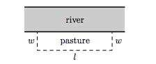
We are tasked to find the dimensions of the pasture which would give a maximum area. We let $w$ denote the width of the pasture and we let $l$ denote the length of the pasture. Since the units given to us in the statement of the problem are feet, we assume $w$ and $l$ are measured in feet. The area of the pasture, which we'll call $A$, is related to $w$ and $l$ by the equation $A = wl$. Since $w$ and $l$ are both measured in feet, $A$ has units of $\text{feet}^2$, or square feet. We are given the total amount of fencing available is $200$ feet, which means $w + l + w = 200$, or, $l+2w = 200$. We now have two equations, $A = wl$ and $l+2w = 200$. In order to use the tools given to us in this section to $\textit{maximize}$ $A$, we need to use the information given to write $A$ as a function of just $\textit{one}$ variable, either $w$ or $l$. This is where we use the equation $l+2w = 200$. Solving for $l$, we find $l = 200-2w$, and we substitute this into our equation for $A$. We get $A = wl = w(200-2w) = 200w-2w^2$. We now have $A$ as a function of $w$, $A(w) = 200w-2w^2 = -2w^2+200w$.

Before we go any further, we need to find the applied domain of $A$ so that we know what values of $w$ make sense in this problem situation.\footnote{Donnie would be very upset if, for example, we told him the width of the pasture needs to be $-50$ feet.} Since $w$ represents the width of the pasture, $w > 0$. Likewise, $l$ represents the length of the pasture, so $l = 200-2w > 0$. Solving this latter inequality, we find $w < 100$. Hence, the function we wish to maximize is $A(w) = -2w^2 + 200w$ for $0 < w < 100$. Since $A$ is a quadratic function (of $w$), we know that the graph of $y = A(w)$ is a parabola. Since the coefficient of $w^2$ is $-2$, we know that this parabola opens downwards. This means that there is a maximum value to be found, and we know it occurs at the vertex. Using the vertex formula, we find $w = -\frac{200}{2(-2)} = 50$, and $A(50) = -2(50)^2 + 200(50) = 5000$. Since $w=50$ lies in the applied domain, $0 < w < 100$, we have that the area of the pasture is maximized when the width is $50$ feet. To find the length, we use $l = 200-2w$ and find $l = 200-2(50) = 100$, so the length of the pasture is $100$ feet. The maximum area is $A(50) = 5000$, or $5000$ square feet. If an average alpaca requires 25 square feet of pasture, Donnie can raise $\frac{5000}{25} = 200$ average alpaca. $\Box$

We conclude this section with the graph of a more complicated absolute value function.

Example $\PageIndex{5}$:

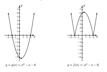
Graph $f(x) = |x^2 - x - 6|$.

Solution

Using the definition of absolute value, Definition 2.4, we have

$$f(x) = \left\{ \begin{array}{rcl} -\left(x^2 - x - 6\right), & \mbox{if} & x^2 - x - 6 < 0 \\ x^2 - x - 6, & \mbox{if} & x^2 - x - 6 \geq 0 \\ \end{array} \right.$$

The trouble is that we have yet to develop any analytic techniques to solve nonlinear inequalities such as $x^2 - x - 6 < 0$. You won't have to wait long; this is one of the main topics of Section 2.4.

Nevertheless, we can attack this problem graphically. To that end, we graph $y = g(x) = x^2 - x-6$ using the intercepts and the vertex. To find the $x$-intercepts, we solve $x^2 - x - 6 = 0$. Factoring gives $(x-3)(x+2)=0$ so $x=-2$ or $x=3$. Hence, $(-2,0)$ and $(3,0)$ are $x$-intercepts. The $y$-intercept $(0,-6)$ is found by setting $x=0$. To plot the vertex, we find $x = -\frac{b}{2a} = -\frac{-1}{2(1)} = \frac{1}{2}$, and $y = \left(\frac{1}{2}\right)^2 - \left(\frac{1}{2}\right)-6 = -\frac{25}{4} = -6.25$. Plotting, we get the parabola seen below on the left. To obtain points on the graph of $y = f(x) = |x^2-x-6|$, we can take points on the graph of $g(x) = x^2-x-6$ and apply the absolute value to each of the $y$ values on the parabola. We see from the graph of $g$ that for $x \leq -2$ or $x \geq 3$, the $y$ values on the parabola are greater than or equal to zero (since the graph is on or above the $x$-axis), so the absolute value leaves these portions of the graph alone. For $x$ between $-2$ and $3$, however, the $y$ values on the parabola are negative. For example, the point $(0,-6)$ on $y = x^2-x-6$ would result in the point $(0,|-6|) = (0,-(-6))= (0,6)$ on the graph of $f(x) = |x^2-x-6|$. Proceeding in this manner for all points with $x$-coordinates between $-2$ and $3$ results in the graph seen below on the right.

If we take a step back and look at the graphs of $g$ and $f$ in the last example, we notice that to obtain the graph of $f$ from the graph of $g$, we reflect a portion of the graph of $g$ about the $x$-axis. We can see this analytically by substituting $g(x) = x^2-x-6$ into the formula for $f(x)$ and calling to mind Theorem 1.4 from Section 1.7.

$$f(x) = \left\{ \begin{array}{rcl} -g(x), & \mbox{if} & g(x) < 0 \\ g(x), & \mbox{if} & g(x) \geq 0 \\ \end{array} \right.$$

The function $f$ is defined so that when $g(x)$ is negative (i.e., when its graph is below the $x$-axis), the graph of $f$ is its refection across the $x$-axis. This is a general template to graph functions of the form $f(x) = |g(x)|$. From this perspective, the graph of $f(x) = |x|$ can be obtained by reflection the portion of the line $g(x) =x$ which is below the $x$-axis back above the $x$-axis creating the characteristic `$\vee$' shape.