6.2: Vectors from an Algebraic Point of View

Focus Questions

The following questions are meant to guide our study of the material in this section. After studying this section, we should understand the concepts motivated by these questions and be able to write precise, coherent answers to these questions.

• How do we find the component form of a vector?
• How do we find the magnitude and the direction of a vector written in component form?
• How do we add and subtract vectors written in component form and how do we find the scalar product of a vector written in component form?
• What is the dot product of two vectors?
• What does the dot product tell us about the angle between two vectors?
• How do we find the projection of one vector onto another?

Introduction and Terminology

We have seen that a vector is completely determined by magnitude and direction. So two vectors that have the same magnitude and direction are equal. That means that we can position our vector in the plane and identify it in different ways. For one, we can place the tip of a vector \(\textbf{v}\) at the origin and the tail will wind up at some point \((v_{1}, v_{2})\) as illustrated in Figure \(\PageIndex{1}\).

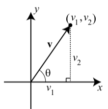
Figure \(\PageIndex{1}\): A Vector in Standard Position

A vector with its initial point at the origin is said to be in standard position and is represent by \(\textbf{v} = \langle v_{1}, v_{2} \rangle\). Please note the important distinction in notation between the vector \(\textbf{v} = \langle v_{1}, v_{2} \rangle\) and the point \((v_{1}, v_{2})\). The coordinates of the terminal point \((v_{1}, v_{2})\) are called the components of the vector \(\textbf{v}\). We call \(\textbf{v} = \langle v_{1}, v_{2} \rangle\) the component form of the vector \(\textbf{v}\). The first coordinate \(\textbf{v}_{1}\) is called the \(x\)-component or the horizontal component of the vector \(\textbf{v}\), and the first coordinate \(\textbf{v}_{2}\) is called the \(y\)-component or the vertical component of the vector \(\textbf{v}\). The nonnegative angle \(\theta\) between the vector and the positive \(x\)-axis (with \(0 \leq \theta \leq 360^\circ\)) is called the direction angle of the vector. See Figure \(\PageIndex{1}\).

Using Basis Vectors

There is another way to algebraically write a vector if the components of the vector are known. This uses the so-called standard basis vectors for vectors in the plane. These two vectors are denoted by \(\textbf{i}\) and \(\textbf{j}\) and are defined as follows and are shown in the diagram below.

\(\textbf{i} = \langle 1, 0 \rangle\) and \(\textbf{j} = \langle 0, 1 \rangle\)

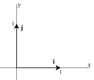
The diagram in Figure \(\PageIndex{2}\) shows how to use the vectors \(\textbf{i}\) and \(\textbf{j}\) to represent a vector \(\textbf{v} = \langle a, b \rangle\).

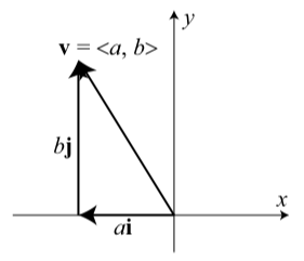
Figure \(\PageIndex{2}\): Using the Vectors \(\textbf{i}\) and \(\textbf{j}\)

The diagram shows that if we place the base of the vector \(\textbf{j}\) at the tip of the vector \(\textbf{i}\), we see that \[\textbf{v} = \langle a, b \rangle = a\textbf{i} + b\textbf{j}\]

This is often called the \(\textbf{i}\), \(\textbf{j}\) form of a vector, and the real number \(a\) is called the \(\textbf{i}\)-component of \(\textbf{v}\) and the real number \(b\) is called the \(\textbf{j}\)-component of \(\textbf{v}\)

Algebraic Formulas for Geometric Properties of a Vector

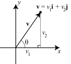
Vectors have certain geometric properties such as length and a direction angle. With the use of the component form of a vector, we can write algebraic formulas for these properties. We will use the diagram to the right to help explain these formulas.

• The magnitude (or length) of the vector \(\textbf{v}\) is the distance from the origin to the point \((v_{1}, v_{2})\) and so \[|\textbf{v}| = \sqrt{v_{1}^{2} + v_{2}^{2}}\]
• The direction angle of \(\textbf{v}\) is, where \(0 \leq \theta < 360^\circ\), and \[\cos(\theta) = \dfrac{v_{1}}{|\textbf{v}|}\] and \[\sin(\theta) = \dfrac{v_{2}}{|\textbf{v}|}\]
• The horizontal and component and vertical component of the vector \(\textbf{v}\) and direction angle \(\theta\) are \[v_{1} = |\textbf{v}|\cos(\theta)\] and \[v_{2} = |\textbf{v}|\sin(\theta)\]

ANOTHER WAY TO LOOK AT THE COMPONENT FORM OF A VECTOR

The component form of a vector represents the vector using two components. \(\vec{u} = \langle x, y \rangle\) indicates the vector represents a displacement of \(x\) units horizontally and \(y\) units vertically.

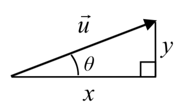
Notice how we can see the magnitude of the vector as the length of the hypotenuse of a right triangle, or in polar form as the radius, \(r\).

ALTERNATE NOTATION FOR VECTOR COMPONENTS

Sometimes you may see vectors written as the combination of unit vectors \(\vec{i}\) and \(\vec{j}\), where \(\vec{i}\) points the right and \(\vec{j}\) points up. In other words, \(\vec{i} = \langle 1, 0 \rangle\) and \(\vec{j} = \langle \theta, 1 \rangle\).

In this notation, the vector \(\vec{u} = \langle 3, -4 \rangle\) would be written as \(\vec{u} = 3\vec{i} - 4\vec{j}\) since both indicate a displacement of 3 units to the right, and 4 units down.

Exercise \(\PageIndex{1}\)

1. Suppose the horizontal component of a vector \(\textbf{v}\) is 7 and the vertical component is \(-3\). So we have \(\textbf{v} = 7\textbf{i} + (-3)\textbf{j} = 7\textbf{i} - 3\textbf{j}\). Determine the magnitude and the direction angle of \(\textbf{v}\).
2. Suppose a vector \(\textbf{w}\) has a magnitude of 20 and a direction angle of \(-200^\circ\). Determine the horizontal and vertical components of \(\textbf{w}\) and write \(\textbf{w}\) in \(\textbf{i}\), \(\textbf{j}\) form.

Answer

1. \(\textbf{v} = 7\textbf{i} + (-3)\textbf{j}\). So \(|\textbf{v}| = \sqrt{7^{2} + (-3)^{2}} = \sqrt{58}\). In addition, \[\cos(\theta) = \dfrac{7}{\sqrt{58}}\space\text{and}\space\sin(\theta) = \dfrac{-3}{\sqrt{58}}\]

So the terminal side of \(\theta\) is in the fourth quadrant, and we can write \[\theta = 360^\circ - \arccos(\dfrac{7}{\sqrt{58}}).\] So \(\theta \approx 336.80^\circ\).

2. We are given \(|\textbf{w}| = 20\) and the direction angle \(\theta\) of \(\textbf{w}\) is \(200^\circ\). So if we write \(\textbf{w} = w_{1}\textbf{i} + w_{2}\textbf{j}\). Then

\[w_{1} = 20\cos(200^\circ) \approx -1.794\]

\[w_{1} = 20\cos(200^\circ) \approx -6.840\]

Operations on Vectors

In pervious sections we earned how to add two vectors and how to multiply a vector by a scalar. At that time, the descriptions of these operations was geometric in nature. We now know about the component form of a vector. So a good question is, “Can we use the component form of vectors to add vectors and multiply a vector by a scalar?”

Figure \(\PageIndex{3}\): The Sum of Vector as Compared to Unit Vector Components

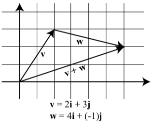
To illustrate the idea above in Figure \(\PageIndex{3}\), remember that a vector added to another vector is arranged tip to tail. Then we draw a new vector from the starting point (tail of first vector) to the ending point (tip of last vector). This new vector is the sum of the two. Although we did not use the component forms of these vectors in the previous section, we can now see that \[\textbf{v} = \langle 2, 3 \rangle = 2\textbf{i} + 3\textbf{j}\] and \[\textbf{w} = \langle 4, -1 \rangle = 4\textbf{i} + (-1)\textbf{j}\]

The diagram above now shows the vectors in a coordinate plane.

Notice that \[\textbf{v} + \textbf{w} = 6\textbf{i} + 2\textbf{j}\] \[\textbf{v} + \textbf{w} = (2 + 4)\textbf{i} + (3 + (-1))\textbf{j}\]

This means that we can add two vectors by adding their horizontal components and by adding their vertical components. See Figure \(\PageIndex{4}\)

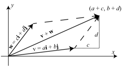
Figure \(\PageIndex{4}\): The Sum of Two Vectors

Exercise \(\PageIndex{2}\)

Let \(\textbf{v} = \langle 3, -2 \rangle\). Draw the vector v in standard position and then draw the vectors \(2\textbf{v}\) and \(-2\textbf{v}\) in standard position. What are the component forms of the vectors \(2\textbf{v}\) and \(-2\textbf{v}\)?

In general, how do you think a scalar multiple of a vector \(\textbf{a} = \langle a_{1}, a_{2} \rangle\) by a scalar \(c\) should be defined? Write a formal definition of a scalar multiple of a vector based on your intuition.

Answer

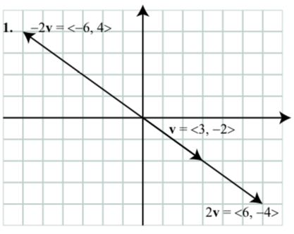
2. For a vector \(\textbf{a} = \langle a_{1}, a_{2} \rangle\) and a scalar \(c\), we define the scalar multiple \(c\textbf{a}\) to be \[c\textbf{a} = \langle ca_{1}, ca_{2} \rangle.\]

Based on the work we have done, we make the following formal definitions.

Definition

For vectors \(\textbf{v} = \langle v_{1}, v_{2} \rangle = v_{1}\textbf{i} + v_{2}\textbf{j}\) and \(\textbf{w} = \langle w_{1}, w_{2} \rangle = w_{1}\textbf{i} + w_{2}\textbf{j}\) and scalar \(c\), we make the following definition:

\[\textbf{v} + \textbf{w} = \langle v_{1} + w_{1}, v_{2} + w_{2}\rangle\]
\[\textbf{v} + \textbf{w} = (v_{1} + w_{1})\textbf{i} + (v_{2} + w_{2})\textbf{j}\]
\[\textbf{v} - \textbf{w} = \langle v_{1} - w_{1}, v_{2} - w_{2}\rangle\]
\[\textbf{v} - \textbf{w} = (v_{1} - w_{1})\textbf{i} + (v_{2} - w_{2})\textbf{j}\]
\[c\textbf{v} = \langle cv_{1}, cv_{2}\rangle\]
\[c\textbf{v} = (cv_{1})\textbf{i} + (cv_{2})\textbf{j}\]

Exercise \(\PageIndex{3}\)

Let \(\textbf{u} = \langle 1, -2 \rangle\), \(\textbf{u} = \langle 0, 4 \rangle\), and \(\textbf{u} = \langle -5, 7 \rangle\).

1. Determine the component form of the vector \(2\textbf{u} - 3\textbf{v}\).
2. Determine the magnitude and the direction angle for \(2\textbf{u} - 3\textbf{v}\).
3. Determine the component form of the vector u\(\textbf{u} + 2\textbf{v} - 7\textbf{w}\).

Answer

Let \(\textbf{u} = \langle 1, -2 \rangle\), and \(\textbf{w} = \langle -5, 7 \rangle\).

1. \(2\textbf{u} - 3\textbf{v} = \langle 2, -4 \rangle - \langle 0, 12 \rangle = \langle 2, -16 \rangle\)

2. \(|2\textbf{u} - 3\textbf{v}| = \sqrt{2^{2} + (-16)^{2}} = \sqrt{260}\). So now let \(\theta\) be the direction angle of \(2\textbf{u} - 3\textbf{v}\). Then

\[\cos(\theta) = \dfrac{2}{\sqrt{260}}\space \text{and} \space \sin(\theta) = \dfrac{-16}{\sqrt{260}}.\]

So the terminal side of \(\theta\) is in the fourth quadfrant. We see that \(\arcsin(\dfrac{-16}{\sqrt{260}}) \approx -82.87^\circ\). Since the direction angle \(\theta\) must satisfy \(a \leq \theta < 360^circ\), we see that \(\theta \approx -82.87^\circ + 360^\circ \approx 277.13^\circ\).

3. \(\textbf{u} + 2\textbf{v} - 7\textbf{w} = \langle 1, -2 \rangle + \langle 0, 8 \rangle - \langle -35, 49 \rangle = \langle 36, -43 \rangle\).

The Dot Product of Two Vectors

Finding optimal solutions to systems is an important problem in applied mathematics. It is often the case that we cannot find an exact solution that satisfies certain constraints, so we look instead for the “best” solution that satisfies the constraints. An example of this is fitting a least squares curve to a set of data like our calculators do when computing a sine regression curve. The dot product is useful in these situations to find “best” solutions to certain types of problems. Although we won’t see it in this course, having collections of perpendicular vectors is very important in that it allows for fast and efficient computations. The dot product of vectors allows us to measure the angle between them and thus determine if the vectors are perpendicular. The dot product has many applications, e.g., finding components of forces acting in different directions in physics and engineering. We introduce and investigate dot products in this section.

We have seen how to add vectors and multiply vectors by scalars, but we have not yet introduced a product of vectors. In general, a product of vectors should give us another vector, but there turns out to be no really useful way to define such a product of vectors. However, there is a dot “product” of vectors whose output is a scalar instead of a vector, and the dot product is a very useful product (even though it isn’t a product of vectors in a technical sense).

Recall that the magnitude (or length) of the vector \(\textbf{u} = \langle u_{1}, u_{2} \rangle\) is: \[|\textbf{u}| = \sqrt{u_{1}^{2} + u_{2}^{2}} = \sqrt{u_{1}u_{1} + u_{2}u_{2}}\]

The expression under the second square root is an important one and we extend it and give it a special name.

Definition

Let \(\textbf{u} = \langle u_{1}, u_{2} \rangle\) and \(\textbf{v} = \langle v_{1}, v_{2} \rangle\) be vectors in the plane. The dot product of \(\textbf{u}\) and \(\textbf{v}\) is the scalar \[\textbf{u}\cdot \textbf{v} = u_{1}v_{1} + u_{2}v_{2}.\]

This may seem like a strange number to compute, but it turns out that the dot product of two vectors is useful in determining the angle between two vectors. Recall we can use the Law of Cosines to determine the sum of two vectors and then used the Law of Sines to determine the angle between the sum and one of those vectors. We have now seen how much easier it is to compute the sum of two vectors when the vectors are in component form. The dot product will allow us to determine the cosine of the angle between two vectors in component form. This is due to the following result:

The Dot Product and the Angle between Two Vectors

If \(\theta\) is the angle between two nonzero vectors \(\textbf{u}\) and \(\textbf{v}\) (\(0^\circ \leq \theta \leq 180^\circ\)), then

\[\textbf{u}\cdot \textbf{v} = |\textbf{u}||\textbf{v}|\cos(\theta)\] or \[\cos(\theta) = \dfrac{\textbf{u}\cdot \textbf{v}}{|\textbf{u}||\textbf{v}|}\]

Notice that if we have written the vectors \(\textbf{v}\) and \(\textbf{w}\) in component form, then we have formulas to compute \(|\textbf{v}|, |\textbf{w}|\), and \(\textbf{v}\cdot \textbf{w}\). This result may seem surprising but it is a fairly direct consequence of the Law of Cosines as we will now show. Let \(\theta\) be the angle between \(\textbf{u}\) and \(\textbf{v}\) as illustrated in Figure \(\PageIndex{5}\)

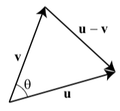
Figure \(\PageIndex{5}\): The angle between \(\textbf{u}\) and \(\textbf{v}\)

We can apply the Law of Cosines to determine the angle \(\theta\) as follows:

\[|\textbf{u} - \textbf{v}|^{2} = |\textbf{u}|^{2} + |\textbf{v}|^{2} - 2|\textbf{u}||\textbf{v}|\cos(\theta)\]
\[(\textbf{u} - \textbf{v})\cdot (\textbf{u} - \textbf{v}) = |\textbf{u}|^{2} + |\textbf{v}|^{2} - 2|\textbf{u}||\textbf{v}|\cos(\theta)\]
\[(\textbf{u} \cdot \textbf{u}) -2(\textbf{u} \cdot \textbf{v}) + (\textbf{v} \cdot \textbf{v})= |\textbf{u}|^{2} + |\textbf{v}|^{2} - 2|\textbf{u}||\textbf{v}|\cos(\theta)\]
\[|\textbf{u}|^{2} -2(\textbf{u} \cdot \textbf{v}) + |\textbf{v}|^{2}= |\textbf{u}|^{2} + |\textbf{v}|^{2} - 2|\textbf{u}||\textbf{v}|\cos(\theta)\]
\[-2(\textbf{u} \cdot \textbf{u}) = -2|\textbf{u}||\textbf{v}|\cos(\theta)\]
\[\textbf{u} \cdot \textbf{u} = |\textbf{u}||\textbf{v}|\cos(\theta)\]

Exercise \(\PageIndex{4}\)

1. Determine the angle \(\theta\) between the vectors \(\textbf{u} = 3\textbf{i} + \textbf{j}\) and \(\textbf{v} = -5\textbf{i} + 2\textbf{j}\).

2. Determine all vectors perpendicular to \(\textbf{u} = \langle 1, 3 \rangle\). How many such vectors are there? Hint: Let \(\textbf{v} = \langle a, b \rangle\). Under what conditions will the angle between \(\textbf{u}\) and \(\textbf{v}\) be \(90^\circ\)?

Answer

1. If \(\theta\) is the angle between \(\textbf{u} = 3\textbf{i} + \textbf{j}\) and \(\textbf{v} = -5\textbf{i} + 2\textbf{j}\), then

\[\cos(\theta) = \dfrac{\textbf{u}\cdot\textbf{v}}{|\textbf{u}||\textbf{v}|} = \dfrac{-13}{\sqrt{10}\sqrt{29}}\]

\[\theta = \cos^{-1}( \dfrac{-13}{\sqrt{10}\sqrt{29}})\]

so \(\theta \approx 139.764^\circ\).

2. If \(\textbf{v} = \langle a, b \rangle\) is perpendicular to \(\textbf{u} = \langle 1, 3 \rangle\), then the angle \(\theta\) between them is \(90^\circ\) and so \(\cos(\theta) = 0\). So we must have \(\textbf{u}\cdot\textbf{v} = 0\) and this means that \(a + 3b = 0\). So any vector \(\textbf{v} = \langle a, b \rangle\) where \(a = -3b\) will be perpendicular to \(\textbf{v}\), and there are infinitely many such vectors. One vector perpendicular to \(\textbf{u}\) is \(\langle -3, 1 \rangle\).

One purpose of Progress Check 3.34 was to use the formula \[\cos(\theta) = \dfrac{\textbf{u}\cdot \textbf{v}}{|\textbf{u}||\textbf{v}|}\]

to determine when two vectors are perpendicular. Two vectors \(\textbf{u}\) and \(\textbf{v}\) will be perpendicular if and only if the angle \(\theta\) between them is \(90^\circ\). Since \(\cos(90^\circ) = 0\), we see that this formula implies that \(\textbf{u}\) and \(\textbf{v}\) will be perpendicular if and only if \(\textbf{u}\cdot \textbf{v} = 0\) (This is because a fraction will be equal to \(0\) only when the numerator is equal to \(0\) and the denominator is not zero.) So we have:

Two vectors are perpendicular if and only if their dot product is equal to \(0\).

Note

When two vectors are perpendicular, we also say that they are orthogonal.

Projections

Another useful application of the dot product is in finding the projection of one vector onto another. An example of where such a calculation is useful is the following.

Usain Bolt from Jamaica excited the world of track and field in 2008 with his world record performances on the track. Bolt won the 100 meter race in a world record time of 9.69 seconds. He has since bettered that time with a race of 9.58 seconds with a wind assistance of 0.9 meters per second in Berlin on August 16, 20092. The wind assistance is a measure of the wind speed that is helping push the runners down the track. It is much easier to run a very fast race if the wind is blowing hard in the direction of the race. So that world records aren’t dependent on the weather conditions, times are only recorded as record times if the wind aiding the runners is less than or equal to 2 meters per second. Wind speed for a race is recorded by a wind gauge that is set up close to the track. It is important to note, however, that weather is not always as cooperative as we might like. The wind does not always blow exactly in the direction of the track, so the gauge must account for the angle the wind makes with the track.

If the wind is blowing in the direction of the vector \(\textbf{u}\) and the track is in the direction of the vector \(\textbf{v}\) in Figure \(\PageIndex{6}\), then only part of the total wind vector is actually working to help the runners.

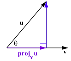
Figure \(\PageIndex{6}\): The Projection of \(\textbf{u}\) onto \(\textbf{v}\)

This part is called the projection of the vector \(\textbf{u}\) onto the vector \(\textbf{v}\) and is denoted \(\textbf{proj}_\textbf{v}\textbf{u}\).

We can find this projection with a little trigonometry. To do so, we let \(\theta\) be the angle between \(\textbf{u}\) and \(\textbf{v}\) as shown in Figure \(\PageIndex{5}\). Using right triangle trigonometry, we see that \[|\textbf{proj}_\textbf{v}\textbf{u}| = |\textbf{u}|\cos(\theta) = |\textbf{u}|\dfrac{\textbf{u}\cdot \textbf{v}}{|\textbf{u}||\textbf{v}|} = \dfrac{\textbf{u}\cdot \textbf{v}}{|\textbf{v}|}\]
The quantity we just derived is called the scalar projection (or component) of \(\textbf{u}\) onto \(\textbf{v}\) and is denoted by \(\textbf{comp}_\textbf{v}\textbf{u}\). Thus \(\textbf{comp}_\textbf{v}\textbf{u} = \dfrac{\textbf{u}\cdot \textbf{v}}{|\textbf{v}|}\)
This gives us the length of the vector projection. So to determine the vector, we use a scalar multiple of this length times a unit vector in the same direction, which is \(\dfrac{1}{|\textbf{v}|}\textbf{v}\). So we obtain

\[\textbf{proj}_\textbf{v}\textbf{u} =|\textbf{proj}_\textbf{v}\textbf{u}|(\dfrac{1}{|\textbf{v}|}) = \dfrac{\textbf{u}\cdot \textbf{v}}{|\textbf{v}|}(\dfrac{1}{|\textbf{v}|}) = \dfrac{\textbf{u}\cdot \textbf{v}}{|\textbf{v}|^{2}}\textbf{v}\]

We can also write the projection of \(\textbf{u}\) onto \(\textbf{v}\) as

\[\textbf{proj}_\textbf{v}\textbf{u} = \dfrac{\textbf{u}\cdot \textbf{v}}{|\textbf{v}|^{2}}\textbf{v} = \dfrac{\textbf{u}\cdot \textbf{v}}{\textbf{v}\cdot \textbf{v}}\textbf{v}\]

The wind component that acts perpendicular to the direction of \(\textbf{v}\) in Figure \(\PageIndex{7}\) is called the projection of \(\textbf{u}\) orthogonal to \(\textbf{v}\) and is denoted \(\textbf{proj}_{\perp\textbf{v}}\textbf{u}\). Since \(\textbf{u} = \textbf{proj}_{\perp\textbf{v}}\textbf{u} + \textbf{proj}_{\textbf{v}}\textbf{u}\), we have that

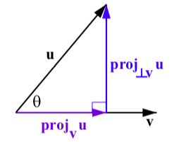
Figure \(\PageIndex{7}\): The Projection of \(\textbf{u}\) onto \(\textbf{v}\)

\[\textbf{proj}_{\perp\textbf{v}}\textbf{u} = \textbf{u} - \textbf{proj}_{\textbf{v}}\textbf{u}\]

Following is a summary of the results we have obtained.

For nonzero vectors \(\textbf{u}\) and \(\textbf{v}\), the projection of the vector \(\textbf{u}\) onto the vector \(\textbf{v}\) \(\textbf{proj}_\textbf{v}\textbf{u}\), is given by

\[\textbf{proj}_\textbf{v}\textbf{u} = \dfrac{\textbf{u}\cdot \textbf{v}}{|\textbf{v}|^{2}}\textbf{v} = \dfrac{\textbf{u}\cdot \textbf{v}}{\textbf{v}\cdot \textbf{v}}\textbf{v}\]

See Figure \(\PageIndex{6}\). The projection of \(\textbf{u}\) orthogonal to \(\textbf{v}\), denoted \(\textbf{proj}_{\perp\textbf{v}}\textbf{u}\), is

\[\textbf{proj}_{\perp\textbf{v}}\textbf{u} = \textbf{u} - \textbf{proj}_{\textbf{v}}\textbf{u}\]

We note that \[\textbf{u} = \textbf{proj}_{\perp\textbf{v}}\textbf{u} + \textbf{proj}_{\textbf{v}}\textbf{u}\]

Exercise \(\PageIndex{5}\)

Let \(\textbf{u} = \langle 7, 5 \rangle\) and \(\textbf{v} = \langle 10, -2\rangle\). Determine \(\textbf{proj}_{\textbf{v}}\textbf{u}\) and \(\textbf{proj}_{\perp\textbf{v}}\textbf{u}\), and verify that \(\textbf{u} = \textbf{proj}_{\perp\textbf{v}}\textbf{u} + \textbf{proj}_{\textbf{v}}\textbf{u}\). Draw a picture showing all of the vectors involved in this.

Answer

Let \(\textbf{u} = \langle 7, 5 \rangle\) and \(\textbf{v} = \langle 10, -2\rangle\). Then

\[\textbf{proj}_{v}\textbf{u} = \dfrac{\textbf{u} \cdot \textbf{v}}{\textbf{|v|}^{2}}\textbf{v} = \langle \dfrac{600}{104}, \dfrac{-120}{104} \rangle \approx \langle 5.769, -1.154 \rangle\]
\[\textbf{proj}_{\perp\textbf{v}}\textbf{u} = \textbf{u} - \dfrac{\textbf{u} \cdot \textbf{v}}{\textbf{|v|}^{2}}\textbf{v}= \langle 7, 5 \rangle - \langle \dfrac{600}{104}, \dfrac{-120}{104} \rangle = \langle \dfrac{128}{104}, \dfrac{640}{104} \rangle \approx \langle 1.231, 6.154 \rangle\]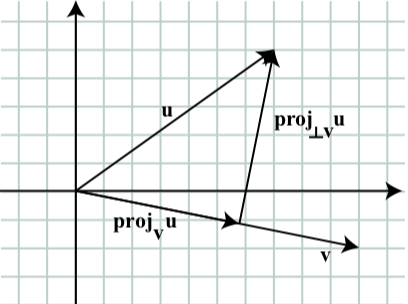

While it can be convenient to think of the vector \(\vec{u} = \langle x, y \rangle\) as an arrow from the origin to the point (\(x\), \(y\)), be sure to remember that most vectors can be situated anywhere in the plane, and simply indicate a displacement (change in position) rather than a position.
It is common to need to convert from a magnitude and angle to the component form of the vector and vice versa. Happily, this process is identical to converting from polar coordinates to Cartesian coordinates, or from the polar form of complex numbers to the \(a+bi\) form.

Example Applications

Example \(\PageIndex{1}\)

Find the component form of a vector with length 7 at an angle of 135 degrees.

Solution

Using the conversion formulas \(x = r\cos(\theta)\) and \(y = r\sin(\theta)\), we can find the components

\[x = 7 \cos (135^{\circ}) = -\dfrac{7\sqrt{2}}{2}\nonumber\]
\[y = 7 \sin (135^{\circ}) = \dfrac{7\sqrt{2}}{2}\nonumber\]

The vector can be written in component form as \(\langle -\dfrac{7\sqrt{2}}{2}, \dfrac{7\sqrt{2}}{2} \rangle\)

Example \(\PageIndex{2}\)

Find the magnitude and angle \(\theta\) representing the vector \(\vec{u} = \langle 3, -2 \rangle\).

Solution

First we can find the magnitude by remembering the relationship between \(x\), \(y\) and \(r\):

\[r^2 = 3^2 + (-2)^2 = 13\nonumber\]
\[r = \sqrt{13}\nonumber\]

Second we can find the angle. Using the tangent,

\[\tan(\theta) = \dfrac{-2}{3}\nonumber\]
\[\theta = \tan^{-1}(-\dfrac{2}{3}) \approx -33.69^{\circ}\nonumber\]or written as a coterminal positive angle, \(326.31^{\circ}\). This angle is in the \(4^{\text{th}}\) quadrant as desired.

Example \(\PageIndex{3}\)

Using vector \(\vec{v}\) from the first Exercise, the vector that travels from the origin to the point (3, 5), find the components, magnitude and angle \(\theta\) that represent this vector.

Answer

\[\vec{v} = \langle 3, 5 \rangle \nonumber\]
\[\text{magnitude} = \sqrt{34}\nonumber\]
\[\theta = \tan^{-1} (\dfrac{5}{3}) = 59.04^{\circ}\nonumber\]

In addition to representing distance movements, vectors are commonly used in physics and engineering to represent any quantity that has both direction and magnitude, including velocities and forces.

Example \(\PageIndex{4}\)

An object is launched with initial velocity 200 meters per second at an angle of 30 degrees. Find the initial horizontal and vertical velocities.

Solution

By viewing the initial velocity as a vector, we can resolve the vector into horizontal and vertical components.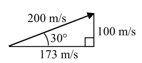

\[x = 200 \cos(30^{\circ} = 200 \cdot \dfrac{\sqrt{3}}{2} \approx 173.205\text{ m/sec}\nonumber\]
\[y = 200 \sin(30^{\circ} = 200 \cdot \dfrac{1}{2} = 100\text{ m/sec}\nonumber\]

This tells us that, absent wind resistance, the object will travel horizontally at about 173 meters each second. Gravity will cause the vertical velocity to change over time – we’ll leave a discussion of that to physics or calculus classes.

Adding and Scaling Vectors in Component Form

To add vectors in component form, we can simply add the corresponding components. To scale a vector by a constant, we scale each component by that constant.

COMBINING VECTORS IN COMPONENT FORM

To add, subtract, or scale vectors in component form

If \(\vec{u} = \langle u_1, u_2 \rangle\), \(\vec{v} = \langle v_1, v_2 \rangle\), and \(c\) is any constant, then

\[\vec{u} + \vec{v} = \langle u_1 + v_1, u_2 + v_2 \rangle\]
\[\vec{u} - \vec{v} = \langle u_1 - v_1, u_2 - v_2 \rangle\]
\[c\vec{u} = \langle cu_1, cu_2 \rangle\]

Example \(\PageIndex{5}\)

Given \(\vec{u} = \langle 3, -2 \rangle\) and \(\vec{v} = \langle -1, 4 \rangle\), find a new vector \(\vec{w} = 3\vec{u} - 2\vec{v}\)

Solution

Using the vectors given,

\[\begin{array} {rcl} {\vec{w}} &= & {3\vec{u} - 2\vec{v}} \\ {} &= & {3 \langle 3, -2 \rangle - 2\langle -1, 4 \rangle \ \ \ \ \ \ \ \ \ \ \ \ \ \ \ \ \ \ \ \ \ \ \text{Scale each vector}} \\ {} &= & {\langle 9, -6 \rangle - \langle -2, 8 \rangle \ \ \ \ \ \ \ \ \ \ \ \ \ \ \ \ \ \ \ \ \ \ \text{Subtract corresponding components}} \\ {} &= & {\langle 11, -14 \rangle} \end{array}\nonumber\]

By representing vectors in component form, we can find the resulting displacement vector after a multitude of movements without needing to draw a lot of complicated non- right triangles. For a simple example, we revisit the problem from the opening of the section. The general procedure we will follow is:

1) Convert vectors to component form
2) Add the components of the vectors
3) Convert back to length and direction if needed to suit the context of the question

Example \(\PageIndex{6}\)

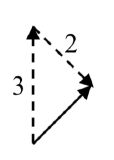
A woman leaves home, walks 3 miles north, then 2 miles southeast. How far is she from home, and what direction would she need to walk to return home? How far has she walked by the time she gets home?

Solution

Let’s begin by understanding the question in a little more depth. When we use vectors to describe a traveling direction, we often position thin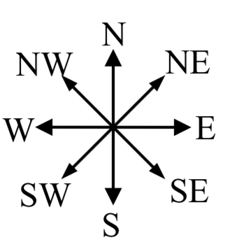gs so north points in the upward direction, east points to the right, and so on, as pictured here.

Consequently, travelling NW, SW, NE or SE, means we are travelling through the quadrant bordered by the given directions at a 45 degree angle.

With this in mind, we begin by converting each vector to components.

A walk 3 miles north would, in components, be \(\langle 0, 3 \rangle\).

A walk of 2 miles southeast would be at an angle of \(45^{\circ}\) South of East. Measuring from standard position the angle would be \(315^{\circ}\).

Converting to components, we choose to use the standard position angle so that we do not have to worry about whether the signs are negative or positive; they will work out automatically.

\[\langle 2\cos (315^{\circ}),\: 2\sin (315^{\circ })\rangle = \langle 2\cdot\frac{\sqrt{2}}{2},\:2\cdot\frac{-\sqrt{2}}{2}\rangle\approx\langle 1.414, -1.414\rangle\nonumber\]

Adding these vectors gives the sum of the movements in component form

\[\langle 0, 3 \rangle + \langle 1.414, -1.414 \rangle = \langle 1.414 1.586 \rangle\nonumber\]

To find how far she is from home and the direction she would need to walk to return home, we could find the magnitude and angle of this vector.

\[\text{Length} = \sqrt{1.414^2 + 1.586^2} = 2.125\nonumber\]

To find the angle, we can use the tangent

\[\tan(\theta) = \dfrac{1.586}{1.414}\nonumber\]
\[\theta = tan^{-1} (\dfrac{1.586}{1.414}) = 48.273^{\circ}\text{ north of east}\nonumber\]

Of course, this is the angle from her starting point to her ending point. To return home, she would need to head the opposite direction, which we could either describe as \(180^{\circ} + 48.273^{\circ} = 228.273^{\circ}\) measured in standard position, or as \(48.273^{\circ}\) south of west (or \(41.727^{\circ}\) west of south).

She has walked a total distance of 3 + 2 + 2.125 = 7.125 miles.

Keep in mind that total distance traveled is not the same as the length of the resulting displacement vector or the “return” vector.

Example \(\PageIndex{7}\)

In a scavenger hunt, directions are given to find a buried treasure. From a starting point at a flag pole you must walk 30 feet east, turn 30 degrees to the north and travel 50 feet, and then turn due south and travel 75 feet. Sketch a picture of these vectors, find their components, and calculate how far and in what direction you must travel to go directly to the treasure from the flag pole without following the map.

Answer

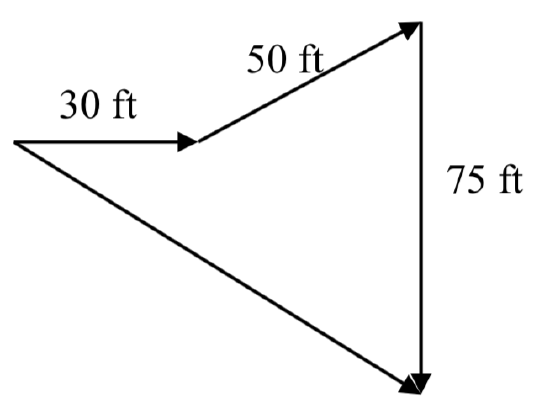
\[\vec{v}_1 = \langle 30, 0 \rangle\quad \vec{v}_2 = \langle 50\cos(30^{\circ}), 50\sin(30^{circ}) \rangle\quad \vec{v}_3 = \langle 0, -75 \rangle\nonumber\]
\[\vec{v}_f = \langle 30 + 50 \cos(30^{\circ}), 50 \sin(30^{\circ}) - 75 \rangle = \langle 73.301, -50 \rangle\nonumber\]
Magnitude = 88.73 feet at an angle of \(34.3^{\circ}\) south of east.

While using vectors is not much faster than using law of cosines with only two movements, when combining three or more movements, forces, or other vector quantities, using vectors quickly becomes much more efficient than trying to use triangles.

Example \(\PageIndex{8}\)

Three forces are acting on an object as shown below, each measured in Newtons (N). What force must be exerted to keep the object in equilibrium (where the sum of the forces is zero)?

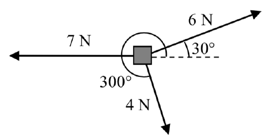
Solution

We start by resolving each vector into components.

The first vector with magnitude 6 Newtons at an angle of 30 degrees will have components

\[\langle 6\cos(30^{\circ}). 6\sin(30^{\circ}) \rangle = \langle 6 \cdot \dfrac{\sqrt{3}}{2}, 6 \cdot \dfrac{1}{2} \rangle = \langle 3\sqrt{3} 3 \rangle\nonumber\]

The second vector is only in the horizontal direction, so can be written as \(\langle -7, 0 \rangle\).

The third vector with magnitude 4 Newtons at an angle of 300 degrees will have components

\[\langle 4 \cos(300^{\circ}), 4\sin(300^{\circ}) \rangle = \langle 4 \cdot \dfrac{1}{2}, 4 \cdot \dfrac{-\sqrt{3}}{2} \rangle = \langle 2, -2\sqrt{3} \rangle\nonumber\]

To keep the object in equilibrium, we need to find a force vector \(x\), \(y\) so the sum of the four vectors is the zero vector, \(\langle 0, 0 \rangle\).

\[\langle 3\sqrt{3}, 3 \rangle + \langle -7, 0 \rangle + \langle 2, -2\sqrt{3} \rangle + \langle x, y \rangle = \langle 0, 0 \rangle\nonumber\]Add component-wise
\[\langle 3\sqrt{3} - 7 + 2, 3 + 0 - 2\sqrt{3} \rangle + \langle x, y \rangle = \langle 0, 0 \rangle\nonumber\]Simplify
\[\langle 3\sqrt{3} - 5, 3 - 2\sqrt{3} \rangle + \langle x, y \rangle = \langle 0, 0 \rangle\nonumber\]Solve
\[\langle x, y \rangle = \langle 0, 0 \rangle - \langle 3\sqrt{3} - 5, 3 - 2\sqrt{3} \rangle\nonumber\]
\[\langle x, y \rangle = \langle -3\sqrt{3} + 5, -3 + 2\sqrt{3} \rangle \approx \langle -0.196, 0.464 \rangle\nonumber\]

This vector gives in components the force that would need to be applied to keep the object in equilibrium. If desired, we could find the magnitude of this force and direction it would need to be applied in.

\[\text{Magnitude} = \sqrt{(-0.196)^2 + 0.464^2} = 0.504\text{ N}\nonumber\]

Angle:

\[\tan(\theta) = \dfrac{0.464}{-0.196}\nonumber\]
\[\theta = \tan^{-1} (\dfrac{0.464}{-0.196} = -67.089^{\circ}\nonumber\]

This is in the wrong quadrant, so we adjust by finding the next angle with the same tangent value by adding a full period of tangent:

\[\theta = -67.089^{\circ} + 180^{\circ} = 112. 911^{circ}\nonumber\]

To keep the object in equilibrium, a force of 0.504 Newtons would need to be applied at an angle of \(112.911^{\circ}\)

Summary of Section

In this section, we studied the following important concepts and ideas:

The component form of a vector \(\textbf{v}\) is written as \(\textbf{v} = \langle v_{1}, v_{2} \rangle\) and the\(\textbf{i},\textbf{j}\) form of the same vector is \(\textbf{v} = v_{1}\textbf{i} + v_{2}\textbf{j} \). Using this notation, we have

• The magnitude (or length) of the vector \(\textbf{v}\) is \(\textbf{v} = \sqrt{v_{1}^{2} + v_{2}^{2}}\).
• The direction angle of \(\textbf{v}\) is \(\theta\), where \(0^\circ \leq \theta < 360^\circ\), and \[\cos(\theta) = \dfrac{v_{1}}{|\textbf{v}|}\] and \[\sin(\theta) = \dfrac{v_{2}}{|\textbf{v}|}\]
• The horizontal and component and vertical component of the vector \(\textbf{v}\) and direction angle \(\theta\) are \[v_{1} = |\textbf{v}|\cos(\theta)\] and \[v_{2} = |\textbf{v}|\sin(\theta)\]

For two vectors \(\textbf{v}\) and \(\textbf{w}\) with \(\textbf{v} = \langle v_{1}, v_{2} \rangle = v_{1}\textbf{i} + v_{2}\textbf{j}\) and \(\textbf{w} = \langle w_{1}, w_{2} \rangle = w_{1}\textbf{i} + w_{2}\textbf{j}\) and a scalar \(c\):

• \[\textbf{v} + \textbf{w} = \langle v_{1} + w_{1}, v_{2} + w_{2}\rangle = (v_{1} + w_{1})\textbf{i} + (v_{2} + w_{2})\textbf{j}\]
• \[\textbf{v} - \textbf{w} = \langle v_{1} - w_{1}, v_{2} - w_{2}\rangle = (v_{1} - w_{1})\textbf{i} + (v_{2} - w_{2})\textbf{j}\]
• \[c\textbf{v} = \langle cv_{1}, cv_{2}\rangle = (cv_{1})\textbf{i} + (cv_{2})\textbf{j}\]
• The dot product of \(\textbf{v}\) and \(\textbf{w}\) is \(\textbf{u}\cdot \textbf{v} = u_{1}v_{1} + u_{2}v_{2}.\)
• If \(\theta\) is the angle between \(\textbf{v}\) and \(\textbf{w}\), then \[\textbf{u} \cdot \textbf{u} = |\textbf{u}||\textbf{v}|\cos(\theta)\] or \[\cos(\theta) = \dfrac{\textbf{u}\cdot \textbf{v}}{|\textbf{u}||\textbf{v}|}\]
• The projection of the vector \(\textbf{v}\) onto the vector \(\textbf{w}\) \(\textbf{proj}_\textbf{w}\textbf{v}\), is given by

  \[\textbf{proj}_\textbf{w}\textbf{v} = \dfrac{\textbf{v}\cdot \textbf{w}}{|\textbf{w}|^{2}}\textbf{w} = \dfrac{\textbf{v}\cdot \textbf{w}}{\textbf{w}\cdot \textbf{w}}\textbf{w}\]

  The projection of \(\textbf{v}\) orthogonal to \(\textbf{w}\), denoted \(\textbf{proj}_{\perp\textbf{w}}\textbf{v}\), is
  \[\textbf{proj}_{\perp\textbf{w}}\textbf{v} = \textbf{v} - \textbf{proj}_{\textbf{w}}\textbf{v}\]

  We note that \[\textbf{w} = \textbf{proj}_{\perp\textbf{w}}\textbf{v} + \textbf{proj}_{\textbf{w}}\textbf{v}\] See Figure \(\PageIndex{8}\).

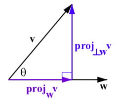
Figure \(\PageIndex{8}\): The Projection of \(\textbf{v}\) onto \(\textbf{w}\)

• Scaling of vectors
• Components of vectors
• Vectors as velocity
• Vectors as forces
• Adding & Scaling vectors in component form - Total distance traveled vs. total displacement