6.3: Solving Systems of Equations with Augmented Matrices

Last updated
Save as PDF

Page ID: 69173

$ \newcommand{\vecs}[1]{\overset { \scriptstyle \rightharpoonup} {\mathbf{#1}} } $ $ \newcommand{\vecd}[1]{\overset{-\!-\!\rightharpoonup}{\vphantom{a}\smash {#1}}} $$\newcommand{\id}{\mathrm{id}}$ $ \newcommand{\Span}{\mathrm{span}}$ $ \newcommand{\kernel}{\mathrm{null}\,}$ $ \newcommand{\range}{\mathrm{range}\,}$ $ \newcommand{\RealPart}{\mathrm{Re}}$ $ \newcommand{\ImaginaryPart}{\mathrm{Im}}$ $ \newcommand{\Argument}{\mathrm{Arg}}$ $ \newcommand{\norm}[1]{\| #1 \|}$ $ \newcommand{\inner}[2]{\langle #1, #2 \rangle}$ $ \newcommand{\Span}{\mathrm{span}}$ $\newcommand{\id}{\mathrm{id}}$ $ \newcommand{\Span}{\mathrm{span}}$ $ \newcommand{\kernel}{\mathrm{null}\,}$ $ \newcommand{\range}{\mathrm{range}\,}$ $ \newcommand{\RealPart}{\mathrm{Re}}$ $ \newcommand{\ImaginaryPart}{\mathrm{Im}}$ $ \newcommand{\Argument}{\mathrm{Arg}}$ $ \newcommand{\norm}[1]{\| #1 \|}$ $ \newcommand{\inner}[2]{\langle #1, #2 \rangle}$ $ \newcommand{\Span}{\mathrm{span}}$$\newcommand{\AA}{\unicode[.8,0]{x212B}}$

Learning Objectives

Be able to describe the definition of an augmented matrix.
Recognize when an augmented matrix would improve the speed at which a system of equations might be solved.
Be able to correctly enter a system of equations into a calculator and interpret the reduced row echelon form of the matrix.

If you have ever solved a system of equations, you know that it can be time intensive and tedious. Fortunately, there is a process by which a calculator can complete the task for you! This section will go over the basic process by which we can solve a system of equations quickly and effectively! This will be particularly helpful for vector questions with tension in a rope or when a mass is hanging from a cable. In this situation there are two tensions and a system of equations is generated to calculate the tension in each rope/cable, where the components are broken out - creating a system of equations.

What is an Augmented Matrix?

Let's first talk about a matrix. For the purposes of this class we will define a matrix to have rows and columns. The rows of the matrix will be associated with the coefficients of each term in an equation. When working with matrices, we must always place the same terms for each equation in the SAME order; this allows us to assume the variable location and, specifically, which variable we are referencing later in the process without having to write it in every step. Here is an example of a system of equations:

\[\begin{align}3x+8y&=11\\5x+7y&=35\\\end{align}\]

Notice that the x term coefficients are in the first column and the y term coefficients are in the second column. The third column would be considered the constants or the value that balances the equation. Including the constant as the third column makes this an Augmented Matrix as shown below:

\[\begin{bmatrix}
3 & 8 & 11\\
5 & 7 & 35
\end{bmatrix} \nonumber\]

NOTE: Sometimes you will see the augmented matrix represented by a vertical line, separating the coefficients from the constants column as below, which wordlessly implies it is an augmented matrix.

\begin{bmatrix}
   \begin{array}{cc|c}
       3 & 8 & 11 \\
       5 & 7 & 35 \\
   \end{array}\end{bmatrix}

Matrix Application on a Calculator to Solve a System of Equations

Create a coefficient matrix corresponding to the equation:
- Select 2nd > MATRIX
- Arrow to EDIT then press ENTER
- Enter the number of rows desired then press ENTER
- Enter the the number of columns that are desired then press ENTER
- Enter each value for each location in the matrix in the same way you entered the previous values.
Click 2nd > QUIT
Press 2nd > MATRIX, MATH, and arrow down to “rref” and press ENTER
Press 2nd > MATRIX, arrow down to the matrix you want, and press ENTER
Press ENTER
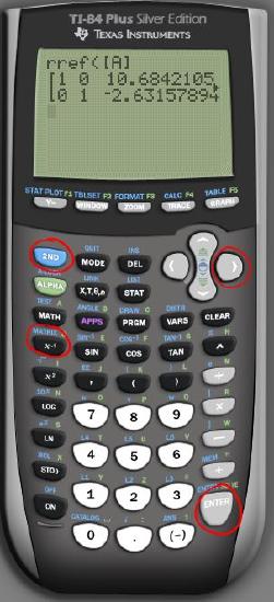
The Row Reduced Matrix should be shown in a diagonal of ones and zeros with the solution to the first "1" corresponds to 10.68... and the second row "1" corresponds to -2.63... .

Notice that in this particular image, the keys used to build the matrix are circled in red - the 2nd button in the top left, the arrow right button in the top right, the Matrix button on the middle left and the enter button in the bottom right.

Example $\PageIndex{1}$

In this scenario a Zipline is VERY loosely attached to two trees. Calculate the tension in the wire supporting the 90.0-kg human. In Figure $\PageIndex{1}$ the free body diagram is shown with angles of 57 degrees and 38 degrees respectively off the horizontal. Remember that if you calculate these components of x and y you will need to use negatives for the x values to the left and y downwards, or in the case of cosine, you will need to use the difference between 180 degrees and 57 degrees.

The arrow downward represents the weight of the human and is not to scale!

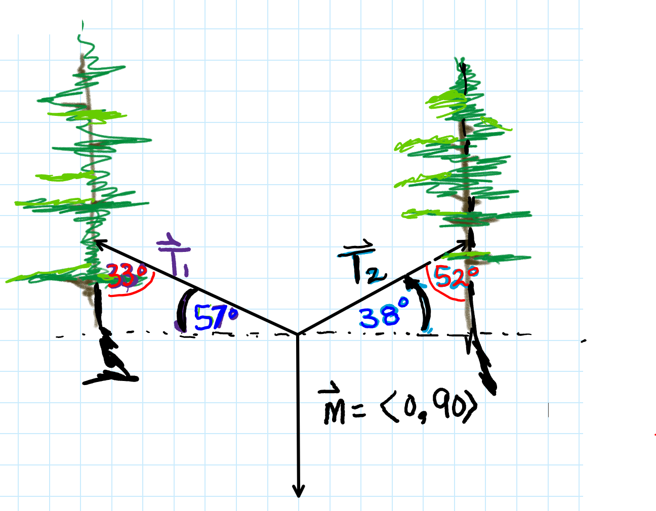$Free Body Diagram in Context.PNG$ Figure $\PageIndex{1}$: Free Body Diagram Sketch of Tension in Cable and Mass of Human Downward

Solution

We need to break down the components into the x direction and the y direction separately.

We will list the equation for the x direction components in the first row and the y direction components in the second row:

\[\begin{align}T1\cos(180^o-57^o)+T2\cos(38^o)& &=0\\T1\sin(180^o-57^o)+T2\sin(38^o)&-90&=0\\\end{align}\]

As an augmented matrix we would have:

\begin{bmatrix}
   \begin{array}{cc|c}
       \cos(123^o) & \cos(38^o) & 0 \\
       \sin(123^o) & \sin(38^o) & 90 \\
   \end{array}\end{bmatrix}

As a row reduced echelon form the tension in the ropes are as follows:

\begin{bmatrix}
\begin{array}{cc|c}
1 & 0 & 71.19187 \\
0 & 1 & 49.20475 \\
\end{array}\end{bmatrix}

Tension $T1=71.19187 kg)$

Tension $T2=49.20475 kg)$

Key Concepts

Augmented matrices are used to quickly solve systems of equations. The columns of the matrix represent the coefficients for each variable present in the system, and the constant on the other side of the equals sign. This implies there will always be one more column than there are variables in the system.
Practice the process of using a matrix to solve a system of equations a few times. This will help with remembering the steps on your calculator - calculators are different. You might need to search for the specific instructions for your calculator. We covered what it looks like when using a TI-84 Plus Silver Edition.
Use the number of equations and the number of variables to determine the appropriate size of the matrix.
When using trig functions within your matrix, be sure to be in the correct mode. If a trig function is negative, be sure to include the sign with the entry.

Glossary

Rows and Columns: a system of equations can be converted into matrix form, where the number of equations is equal to the number of rows and the number of columns is determined by the number of variables plus one more column for the constants on the other side of the equals sign.

Augmented Matrix: a matrix that includes an additional column for the constant term.

Row Reduced Echelon Form: A system of equations in it's simplified or solved form, where diagonals of ones are followed by the corresponding value for each variable in the system's original order.