3.3.2: The Number and Counting System of the Inca Civilization

Background

There is generally a lack of books and research material concerning the historical foundations of the Americas. Most of the “important” information available concentrates on the eastern hemisphere, with Europe as the central focus. The reasons for this may be twofold: first, it is thought that there was a lack of specialized mathematics in the American regions; second, many of the secrets of ancient mathematics in the Americas have been closely guarded.[i] The Peruvian system does not seem to be an exception here. Two researchers, Leland Locke and Erland Nordenskiold, have carried out research that has attempted to discover what mathematical knowledge was known by the Incas and how they used the Peruvian quipu, a counting system using cords and knots, in their mathematics. These researchers have come to certain beliefs about the quipu that we will summarize here.

Counting Boards

It should be noted that the Incas did not have a complicated system of computation. Where other peoples in the regions, such as the Mayans, were doing computations related to their rituals and calendars, the Incas seem to have been more concerned with the simpler task of record-keeping. To do this, they used what are called the “quipu” to record quantities of items. (We will describe them in more detail in a moment.) However, they first often needed to do computations whose results would be recorded on quipu. To do these 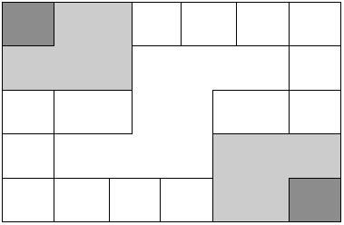computations, they would sometimes use a counting board constructed with a slab of stone. In the slab were cut rectangular and square compartments so that an octagonal (eight-sided) region was left in the middle. Two opposite corner rectangles were raised. Another two sections were mounted on the original surface of the slab so that there were actually three levels available. In the figure shown, the darkest shaded corner regions represent the highest, third level. The lighter shaded regions surrounding the corners are the second highest levels, while the clear white rectangles are the compartments cut into the stone slab.

Pebbles were used to keep accounts and their positions within the various levels and compartments gave totals. For example, a pebble in a smaller (white) compartment represented one unit. Note that there are 12 such squares around the outer edge of the figure. If a pebble was put into one of the two (white) larger, rectangular compartments, its value was doubled. When a pebble was put in the octagonal region in the middle of the slab, its value was tripled. If a pebble was placed on the second (shaded) level, its value was multiplied by six. And finally, if a pebble was found on one of the two highest corner levels, its value was multiplied by twelve. Different objects could be counted at the same time by representing different objects by different colored pebbles.

Example 1

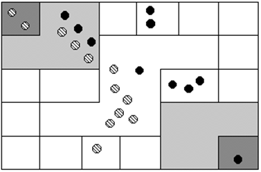
Suppose you have the following counting board with two different kind of pebbles places as illustrated. Let the solid black pebble represent a dog and the striped pebble represent a cat. How many dogs are being represented?

Solution

• There are two black pebbles in the outer square regions…these represent 2 dogs.
• There are three black pebbles in the larger (white) rectangular compartments. These represent 6 dogs.
• There is one black pebble in the middle region…this represents 3 dogs.
• There are three black pebbles on the second level…these represent 18 dogs.
• Finally, there is one black pebble on the highest corner level…this represents 12 dogs.

We then have a total of \(2+6+3+18+12 = 41\) dogs.

Try it Now 1

How many cats are represented on this board?

Answer

\(1+6 \times 3+3 \times 6+2 \times 12=61\) cats.

The Quipu

This kind of board was good for doing quick computations, but it did not provide a good way to keep a permanent recording of quantities or computations. For this purpose, they used the quipu. The quipu is a collection of cords with knots in them. These cords and knots are carefully arranged so that the position and type of cord or knot gives specific information on how to decipher the cord.

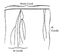
A quipu is made up of a main cord which has other cords (branches) tied to it. See pictures to the right.[ii]

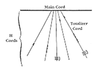Locke called the branches H cords. They are attached to the main cord. B cords, in turn, were attached to the H cords. Most of these cords would have knots on them. Rarely are knots found on the main cord, however, and tend to be mainly on the H and B cords. A quipu might also have a “totalizer” cord that summarizes all of the information on the cord group in one place.

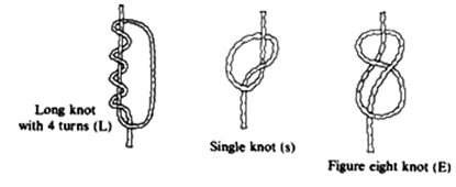Locke points out that there are three types of knots, each representing a different value, depending on the kind of knot used and its position on the cord. The Incas, like us, had a decimal (base-ten) system, so each kind of knot had a specific decimal value. The Single knot, pictured in the middle of the diagram[iii] was used to denote tens, hundreds, thousands, and ten thousands. They would be on the upper levels of the H cords. The figure-eight knot on the end was used to denote the integer “one.” Every other integer from 2 to 9 was represented with a long knot, shown on the left of the figure. (Sometimes long knots were used to represents tens and hundreds.) Note that the long knot has several turns in it…the number of turns indicates which integer is being represented. The units (ones) were placed closest to the bottom of the cord, then tens right above them, then the hundreds, and so on.

In order to make reading these pictures easier, we will adopt a convention that is consistent. For the long knot with turns in it (representing the numbers 2 through 9), we will use the following notation:  

The four horizontal bars represent four turns and the curved arc on the right links the four turns together. This would represent the number 4.

We will represent the single knot with a large dot ( · ) and we will represent the figure eight knot with a sideways eight ( \( \infty \)).

Example 2

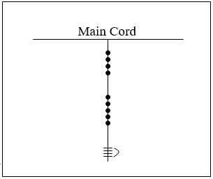What number is represented on the cord shown?

Solution

On the cord, we see a long knot with four turns in it…this represents four in the ones place. Then 5 single knots appear in the tens position immediately above that, which represents 5 tens, or 50. Finally, 4 single knots are tied in the hundreds, representing four 4 hundreds, or 400. Thus, the total shown on this cord is 454.

Try it Now 2

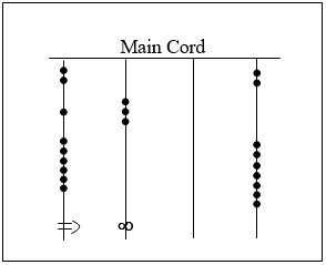What numbers are represented on each of the four cords hanging from the main cord?

Answer

From left to right:
\(\begin{array}{l}
\text { Cord } 1=2,162 \\
\text { Cord } 2=301 \\
\text { Cord } 3=0 \\
\text { Cord } 4=2,070
\end{array}\)

The colors of the cords had meaning and could distinguish one object from another. One color could represent llamas, while a different color might represent sheep, for example. When all the colors available were exhausted, they would have to be re-used. Because of this, the ability to read the quipu became a complicated task and specially trained individuals did this job. They were called Quipucamayoc, which means keeper of the quipus. They would build, guard, and decipher quipus.

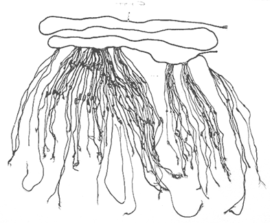As you can see from this photograph of an actual quipu, they could get quite complex.

There were various purposes for the quipu. Some believe that they were used to keep an account of their traditions and history, using knots to record history rather than some other formal system of writing. One writer has even suggested that the quipu replaced writing as it formed a role in the Incan postal system.[iv] Another proposed use of the quipu is as a translation tool. After the conquest of the Incas by the Spaniards and subsequent “conversion” to Catholicism, an Inca supposedly could use the quipu to confess their sins to a priest. Yet another proposed use of the quipu was to record numbers related to magic and astronomy, although this is not a widely accepted interpretation.

The mysteries of the quipu have not been fully explored yet. Recently, Ascher and Ascher have published a book, The Code of the Quipu: A Study in Media, Mathematics, and Culture, which is “an extensive elaboration of the logical-numerical system of the quipu.”[v] For more information on the quipu, you may want to check out the following Internet link:

www.anthropology.wisc.edu/salomon/Chaysimire/khipus.php

We are so used to seeing the symbols 1, 2, 3, 4, etc. that it may be somewhat surprising to see such a creative and innovative way to compute and record numbers. Unfortunately, as we proceed through our mathematical education in grade and high school, we receive very little information about the wide range of number systems that have existed and which still exist all over the world. That’s not to say our own system is not important or efficient. The fact that it has survived for hundreds of years and shows no sign of going away any time soon suggests that we may have finally found a system that works well and may not need further improvement, but only time will tell that whether or not that conjecture is valid or not. We now turn to a brief historical look at how our current system developed over history.

---

[i] Diana, Lind Mae; The Peruvian Quipu in Mathematics Teacher, Issue 60 (Oct., 1967), p. 623-28.

[ii] Diana, Lind Mae; The Peruvian Quipu in Mathematics Teacher, Issue 60 (Oct., 1967), p. 623-28.

[iii] wiscinfo.doit.wisc.edu/chaysimire/titulo2/khipus/what.htm

[iv] Diana, Lind Mae; The Peruvian Quipu in Mathematics Teacher, Issue 60 (Oct., 1967), p. 623-28.

[v] http://www.cs.uidaho.edu/~casey931/seminar/quipu.html