
3.3: Power Functions and Polynomial Functions


- Last updated
- Oct 31, 2021
- Save as PDF
( \newcommand{\kernel}{\mathrm{null}\,}\)
Learning Objectives
- Identify power functions and polynomial functions.
- Identify end behavior of power functions and polynomial functions.
- Identify the degree and leading coefficient of polynomial functions.
Identifying Power Functions
A power function is a function with a single term that is the product of a real number (called a coefficient), and a variable raised to a fixed real number. For example, look at functions for the area of a circle or volume of a sphere with radius r.
A(r)=πr2V(r)=43πr3
Both of these are examples of power functions because they consist of a coefficient, π or 43π, multiplied by a variable r raised to a fixed power.
Definition: Power Function
A power function is a function that can be represented in the form
f(x)=kxp
where parameters k and p are real numbers, k is the coefficient and p is the power of the function.
![]() Is f(x)=2x a power function?
Is f(x)=2x a power function?
No. The variable in a power function is in the base. This function has the variable in the exponent instead, so it is called an exponential function, not a power function.
Example 3.3.1: Identify Equations of Power Functions
Which of the following functions are power functions?
|
f(x)=1Constant functionf(x)=xIdentity functionf(x)=x2Quadratic functionf(x)=x3Cubic function |
f(x)=1xReciprocal functionf(x)=1x2Reciprocal squared functionf(x)=√xSquare root functionf(x)=3√xCube root function |
Solution
All of the listed functions are power functions because they can be written in the form of Equation ???.
- The constant and identity functions are power functions because they can be written as f(x)=x0 and f(x)=x1 respectively.
- The quadratic and cubic functions are power functions with whole number powers f(x)=x2 and f(x)=x3.
- The reciprocal and reciprocal squared functions are power functions with negative whole number powers because they can be written as f(x)=x−1 and f(x)=x−2.
- The square and cube root functions are power functions with fractional powers because they can be written as f(x)=x1/2 or f(x)=x1/3.
![]() Try It 3.3.1
Try It 3.3.1
Which functions are power functions?
- f(x)=2x2⋅4x3
- g(x)=−x5+5x3−4x
- h(x)=2x5−13x2+4
- Answer
-
f(x) is a power function because it can be written as f(x)=8x5. The other functions are not power functions.
Identifying End Behavior of Power Functions
When describing power functions, what happens as numbers get very large is important. To describe the behavior as numbers become larger and larger, we use the idea of infinity. We use the symbol ∞ for positive infinity and −∞ for negative infinity. When we say that “x approaches infinity,” which can be symbolically written as x→∞, we are describing a behavior; we are saying that x is increasing without bound. The behavior of the graph of a function as the magnitude of the input values gets very large (x→−∞ or x→∞) is referred to as the end behavior of the function. We can use words or symbols to describe end behavior.
|
Figure 3.3.2 shows the graphs of f(x)=x2, g(x)=x4 and and h(x)=x6, which are all power functions with even, whole-number powers. Notice that these graphs have similar shapes, very much like that of the quadratic function in the toolkit. However, as the power increases, the graphs flatten somewhat near the origin and become steeper away from the origin. With these even-power functions, as the input increases or decreases without bound, the output values become very large, positive numbers. Equivalently, we could describe this behavior by saying that as x approaches positive or negative infinity, the f(x) values increase without bound. In symbolic form, we could write as x→±∞,f(x)→∞ or limx→±∞(f(x)=∞
|
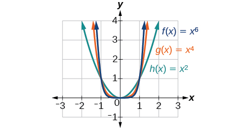 Figure 3.3.2: Even-power functions |
This example and the one below illustrate that functions of the form f(x)=xn reveal symmetry of one kind or another. First, in Figure 3.3.2 above we see that even functions of the form f(x)=xn, n even, are symmetric about the y-axis. In Figure 3.3.3 below we see that odd functions of the form f(x)=xn, n odd, are symmetric about the origin.
|
Figure 3.3.3 shows the graphs of f(x)=x3, g(x)=x5, and h(x)=x7, which are all power functions with odd, whole-number powers. Notice that these graphs look similar to the cubic function in the toolkit. Again, as the power increases, the graphs flatten near the origin and become steeper away from the origin. For these odd power functions, as x approaches negative infinity, f(x) decreases without bound. As x approaches positive infinity, f(x) increases without bound. In symbolic form we write as x→−∞,f(x)→−∞ or limx→−∞f(x)=−∞as x→∞,f(x)→∞ or limx→∞f(x)=∞ |
Figure 3.3.3: Odd-power function |
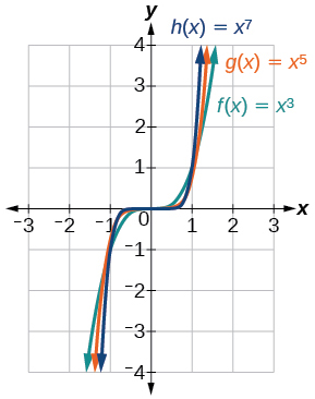
Figure 3.3.4 below shows the end behavior of power functions in the form f(x)=kxn where n is a non-negative integer depending on the power n and the constant coefficient k.
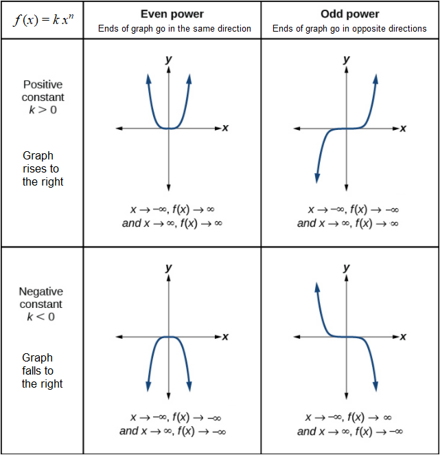
![]() HowTo: Find the end behaviour of a power function f(x)=kxn, n is a non-negative integer.
HowTo: Find the end behaviour of a power function f(x)=kxn, n is a non-negative integer.
- Determine whether the constant coefficient k is positive or negative.
- If positive, the graph rises on the right
- If negative, the graph falls on the right
- Determine whether the power n is even or odd.
- If even, the ends of the graph go in the same direction
- If odd, the ends of the graph go in opposite directions
- The end behaviour analysis can be confirmed by looking at Figure 3.3.4.
Example 3.3.2: Identify End Behavior for an Equation of a Power Function
|
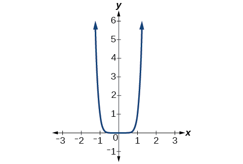
Describe the end behavior of the graph of f(x)=x8. Solution Because the coefficient of the power function is 1 which is positive
Because the exponent of the power function is 8 (an even number)
The graph of the function is shown in Figure 3.3.5. |
|
Example 3.3.3:
|
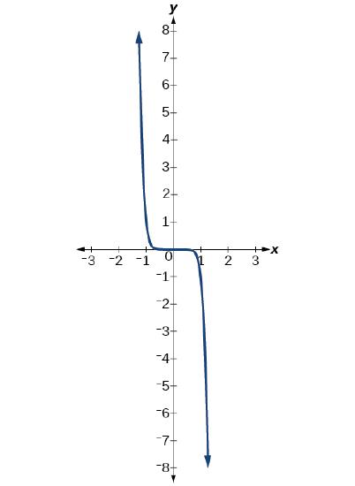
Describe the end behavior of the graph of f(x)=−x9. Solution The exponent of the power function is 9 (an odd number). Because the coefficient (-1) is negative
Because the exponent of the power function is 9 (an odd number)
The graph of the function is shown in Figure 3.3.6. |
|
![]() Try It 3.3.3
Try It 3.3.3
Describe in words and symbols the end behavior of f(x)=−5x4.
- Answer
-
Coefficient −5 is negative, so the graph falls on the right; as x→∞, f(x)→−∞
Power 4 is even, so the ends of the graph go in the same direction (down); as x→−∞, f(x)→−∞
Identifying Polynomial Functions
A polynomial function consists of either zero or the sum of a finite number of non-zero terms, each of which is the product of a number, called the coefficient of the term, and a variable raised to a non-negative integer power.
Definition: Polynomial Functions
Let n be a non-negative integer. A polynomial function is a function that can be written in the form
f(x)=anxn+...+a2x2+a1x+a0
This is called the general form of a polynomial function. Each ai is a coefficient and can be any real number. Each product aixi is a term of a polynomial function. Each exponent is a non-negative integer.
Example 3.3.4: Identify Equations of Polynomial Functions
Which of the following are polynomial functions?
- f(x)=2x3⋅3x+4
- g(x)=−x(x2−4)
- h(x)=5√x+2
Solution
The first two functions are examples of polynomial functions because they can be written in the form of Equation ???, where the powers are non-negative integers and the coefficients are real numbers.
- f(x) can be written as f(x)=6x4+4.
- g(x) can be written as g(x)=−x3+4x.
- h(x) cannot be written in this form and is therefore not a polynomial function.
Identifying Polynomial Graphs
Polynomial functions have graphs that do not have sharp corners; these types of graphs are called smooth. Graphs of polynomial functions also have no breaks. Curves with no breaks are called continuous. The graphs of polynomial functions are both continuous and smooth.
Example 3.3.5: Recognize Graphs of Polynomial Functions
|
Which of the graphs in Figure 3.3.2 represents a polynomial function?
Solution
|
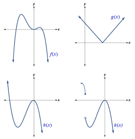 Figure 3.3.2 |
![]() Do all polynomial functions have as their domain all real numbers?
Do all polynomial functions have as their domain all real numbers?
Do all polynomial functions have as their domain all real numbers?
- Yes. Any real number is a valid input for a polynomial function.
Identifying the Degree and Leading Coefficient of a Polynomial Function
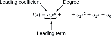
Terminology of Polynomial Functions
|
 |
![]() How To: Given a polynomial function, identify the degree and leading coefficient
How To: Given a polynomial function, identify the degree and leading coefficient
- Find the highest power of x. This is the degree of the polynomial.
- Identify the term containing the highest power of x. This is the leading term.
- Identify the coefficient of the leading term. This is the leading coefficient.
Example 3.3.6: Identify the Degree and Leading Coefficient of a Polynomial Function
Identify the degree, leading term, and leading coefficient of the following polynomial functions.
f(x)=3+2x2−4x3
g(t)=5t5−2t3+7t
h(p)=6p−p3−2
Solution
- For the function f(x), the highest power of x is 3, so the degree is 3. The leading term is the term containing that degree, −4x3. The leading coefficient is the coefficient of that term, −4.
- For the function g(t), the highest power of t is 5, so the degree is 5. The leading term is the term containing that degree, 5t5. The leading coefficient is the coefficient of that term, 5.
- For the function h(p), the highest power of p is 3, so the degree is 3. The leading term is the term containing that degree, −p3; the leading coefficient is the coefficient of that term, −1.
![]() Try It 3.3.7
Try It 3.3.7
Identify the degree, leading term, and leading coefficient of the polynomial f(x)=4x2−x6+2x−5.
- Answer
-
The degree is 6. The leading term is −x6. The leading coefficient is −1.
Identifying End Behavior of Polynomial Equations
Knowing the degree of a polynomial function is useful in helping us predict its end behavior. To determine its end behavior, look at the leading term of the polynomial function. Because the power of the leading term is the highest, that term will grow significantly faster than the other terms as x grows without bound, so its behavior will dominate the graph. For any polynomial, the end behavior of the polynomial will match the end behavior of the term of highest degree. Therefore, the graphs of all polynomial functions will eventually rise or fall without bound when going far to the left or far to the right.
![]() HowTo: Given a polynomial function, find its end behaviour
HowTo: Given a polynomial function, find its end behaviour
|
Schematic Diagram of Polynomial End Behaviour |
Because the end behaviour of a polynomial is determined by its leading term, which is a power function, the end behaviour of a polynomial is the same as that of a power function, as illustrated in Figure 3.3.4.
Example 3.3.8: Given an Equation of a Polynomial Function, State its End Behavior
Given the following polynomial functions, determine its leading term, degree, and end behavior.
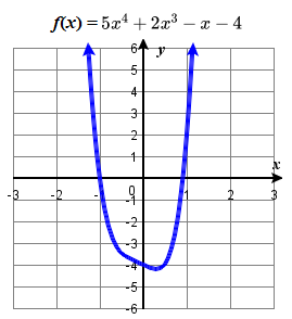
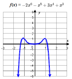
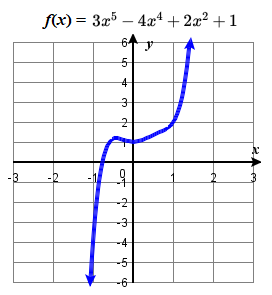
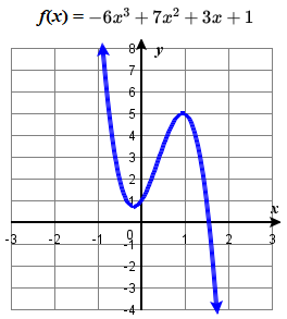
(a) 5x4+2x3−x−4 (b) 3x5−4x4+2x2+1 (c) −2x6−x5+3x4+x3 (d) −6x3+7x2+3x+1
Solution
|
(a) Polynomial Function: 5x4+2x3−x−4 Leading Term: 5x4 (degree 4)
Graph: |
(c) Polynomial Function: −2x6−x5+3x4+x3 Leading Term: −2x6 (degree 6)
Graph: |
|
(b) Polynomial Function: 3x5−4x4+2x2+1 Leading Term: 3x5 (degree 5)
Graph: |
(d) Polynomial Function: −6x3+7x2+3x+1 Leading Term: −6x3 (degree 3)
Graph: |
![]() How to: Given a factored polynomial, determine its leading term
How to: Given a factored polynomial, determine its leading term
- Multiply the high order terms of each of the factors.
- The result is the leading term of the polynomial.
Example 3.3.9
Given the function f(x)=−3x2(x−1)(x+4), determine its leading term, degree, and end behavior.
Solution
One could begin by expanding f(x) to obtain the general form of the polynomial, f(x)=−3x2(x−1)(x+4). HOWEVER, this involves a lot of unnecessary work because the only term of interest is the leading term. The leading term of f(x)=−3x2(x−1)(x+4)=−3x2(x−1)(x+4) is the product of the leading terms in each of the factors. So in this example, the leading term is simply the product −3x2(x)(x)=−3x4. Thus the leading coefficient is negative (–3), so the graph falls to the right …↘ and the degree of the polynomial is 4, which is an even number, so the ends of the graph go in the same direction ( ↙…↘ ), or more formally, as x→−∞,f(x)→−∞ and as x→∞,f(x)→−∞
![]() Try It 3.3.10
Try It 3.3.10
Given the function f(x)=0.2(x−2)(4x+1)3(x−5)3, determine its leading term, degree, and end behavior.
- Answer
-
The leading term is 0.2(x)(4x)3(x)3=12.8x7, so it is a degree 7 polynomial. As x approaches positive infinity, f(x) increases without bound; as x approaches negative infinity, f(x) decreases without bound. (rises to the right, ends in opposite directions: ↙…↗ )
Intercepts of Polynomials
![]() How to: Given a polynomial function, determine its intercepts
How to: Given a polynomial function, determine its intercepts
- Determine the y-intercept by setting x=0 and finding y.
- If the polynomial function is factorable, factor it into a product of linear and irreducible quadratic factors.
- Set each factor equal to zero and solve. The x-intercepts are the solutions (or zeros) that are real numbers.
- A polynomial of degree n has n zeros. Some of these zeros can have the same value; some can be imaginary.
Example 3.3.11: Find Intercepts of a Factored Polynomial
Given the polynomial function f(x)=(x−2)(x+1)(x−4), determine the y-and x-intercepts, the leading term, and the end behaviour.
Solution
The y-intercept occurs when the input is zero, so substitute 0 for x.
f(0)=(0−2)(0+1)(0−4)=(−2)(1)(−4)=8
The y-intercept is (0,8).
The x-intercepts occur when the output is zero.
0=(x−2)(x+1)(x−4)
x−2=0orx+1=0orx−4=0x=2orx=−1orx=4
The x-intercepts are (2,0),(–1,0), and (4,0).
The leading term is (x)(x)(x) = x^3. Therefore the graph rises to the right (positive coefficient) and falls to the left (odd degree so ends go in opposite directions): \swarrow \dots \nearrow
Example \PageIndex{12}
Find the y- and x-intercepts of g(x)=(x−2)^2(2x+3). Find the leading term and describe the end behaviour.
Solution
The y-intercept can be found by evaluating g(0).
\begin{align*} g(0)&=(0−2)^2(2(0)+3) =12 \end{align*}
So the y-intercept is (0,12).
The x-intercepts can be found by solving g(x)=0.
(x−2)^2(2x+3)=0 \nonumber
\begin{align*} (x−2)^2&=0 & & & (2x+3)&=0 \\ x−2&=0 & &\text{or} & x&=−\dfrac{3}{2} \\ x&=2 \end{align*}
So the x-intercepts are (2,0) and \left(−\dfrac{3}{2},0\right).
The leading term is (x)^2(2x)=2x^3. Therefore the graph rises to the right (positive coefficient) and falls to the left (odd degree so ends go in opposite directions): \swarrow \dots \nearrow
Example \PageIndex{13}: Find x-intercepts of a Polynomial Function by Factoring
|
Find the y- and x-intercepts for f(x)=x^3−5x^2−x+5. Solution The y-intercept is (0,5) because f(0)=5. Find solutions for f(x)=0 by factoring. \begin{align*} x^3−5x^2−x+5&=0 &&\text{Factor by grouping.} \\ x^2(x−5)−(x−5)&=0 &&\text{Factor out the common factor.} \\ (x^2−1)(x−5)&=0 &&\text{Factor the difference of squares.} \\ (x+1)(x−1)(x−5)&=0 &&\text{Set each factor equal to zero.} \end{align*} \begin{align*} x+1&=0 & &\text{or} & x−1&=0 & &\text{or} & x−5&=0 \\ x&=−1 &&& x&=1 &&& x&=5\end{align*} There are three x-intercepts: (−1,0), (1,0), and (5,0). |
Figure \PageIndex{13}: Graph of f(x). |
![]() Try It \PageIndex{14}
Try It \PageIndex{14}
Given the polynomial function f(x)=2x^3−6x^2−20x, determine the y- and x-intercepts. Find the leading term and describe the end behaviour.
- Answer
-
y-intercept (0,0); x-intercepts (0,0),(–2,0), and (5,0). The leading term is 2x^3. The curve rises to the right (positive coefficient) and falls to the left (odd degree so ends go in opposite directions): \swarrow \dots \nearrow
![]() Try It \PageIndex{15}
Try It \PageIndex{15}
Find the y- and x-intercepts of the function f(x)=x^4+5x^3−4x^2−20x. Find the leading term and describe the end behaviour.
- Answer
-
- y-intercept (0,0);
- x-intercepts (0,0), (–2,0), (2,0), and (-5,0).
- The leading term is x^4, so the curve rises both on the left and on the right: \nwarrow \dots \nearrow
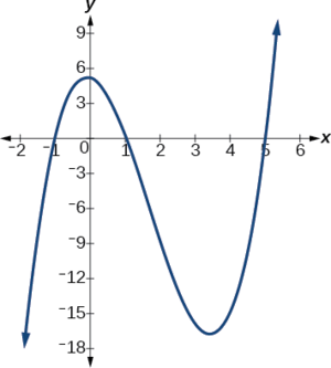
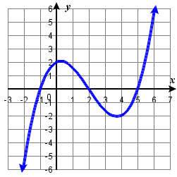
Example \PageIndex{16}: Given a graph of a polynomial, find a possible degree for it
Describe the end behavior and characteristics of the leading term and degree of the polynomial function in the figure below
|
Figure \PageIndex{16}. |
Solution
3. Because there are 3 x-intercepts, the degree is at least three. |
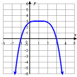
![]() Try It \PageIndex{17}
Try It \PageIndex{17}
|
Describe the end behavior, and characteristics of the leading term and degree of the polynomial function in the Figure below.
|
|
Key Equations
- general form of a polynomial function: f(x)=a_nx^n+a_{n-1}x^{n-1}...+a_2x^2+a_1x+a_0
Key Concepts
- A power function is a variable base raised to a number power.
- The behavior of a graph as the input decreases beyond bound and increases beyond bound is called the end behavior.
- The end behavior depends on whether the power is even or odd and the sign of the leading term.
- A polynomial function is the sum of terms, each of which consists of a transformed power function with positive whole number power.
- The degree of a polynomial function is the highest power of the variable that occurs in a polynomial. The term containing the highest power of the variable is called the leading term. The coefficient of the leading term is called the leading coefficient.
- The end behavior of a polynomial function is the same as the end behavior of the power function that corresponds to the leading term of the function.
Glossary
- coefficient \qquad a nonzero real number multiplied by a variable raised to an exponent
- continuous function \qquad a function whose graph can be drawn without lifting the pen from the paper because there are no breaks in the graph
- degree \qquad the highest power of the variable that occurs in a polynomial
- end behavior \qquad the behavior of the graph of a function as the input decreases without bound and increases without bound
- leading coefficient \qquad the coefficient of the leading term
- leading term \qquad the term containing the highest power of the variable
- polynomial function \qquad a function that consists of either zero or the sum of a finite number of non-zero terms, each of which is a product of a number, called the coefficient of the term, and a variable raised to a non-negative integer power.
- power function \qquad a function that can be represented in the form f(x)=kx^p where k is a constant, the base is a variable, and the exponent, p, is a constant
- smooth curve \qquad a graph with no sharp corners
- term of a polynomial function \qquad any a_ix^i of a polynomial function in the form f(x)=a_nx^n+a_{n-1}x^{n-1}...+a_2x^2+a_1x+a_0