4.7: Exponential and Logarithmic Models

Last updated
Save as PDF

Page ID: 34908

$ \newcommand{\vecs}[1]{\overset { \scriptstyle \rightharpoonup} {\mathbf{#1}} } $ $ \newcommand{\vecd}[1]{\overset{-\!-\!\rightharpoonup}{\vphantom{a}\smash {#1}}} $$\newcommand{\id}{\mathrm{id}}$ $ \newcommand{\Span}{\mathrm{span}}$ $ \newcommand{\kernel}{\mathrm{null}\,}$ $ \newcommand{\range}{\mathrm{range}\,}$ $ \newcommand{\RealPart}{\mathrm{Re}}$ $ \newcommand{\ImaginaryPart}{\mathrm{Im}}$ $ \newcommand{\Argument}{\mathrm{Arg}}$ $ \newcommand{\norm}[1]{\| #1 \|}$ $ \newcommand{\inner}[2]{\langle #1, #2 \rangle}$ $ \newcommand{\Span}{\mathrm{span}}$ $\newcommand{\id}{\mathrm{id}}$ $ \newcommand{\Span}{\mathrm{span}}$ $ \newcommand{\kernel}{\mathrm{null}\,}$ $ \newcommand{\range}{\mathrm{range}\,}$ $ \newcommand{\RealPart}{\mathrm{Re}}$ $ \newcommand{\ImaginaryPart}{\mathrm{Im}}$ $ \newcommand{\Argument}{\mathrm{Arg}}$ $ \newcommand{\norm}[1]{\| #1 \|}$ $ \newcommand{\inner}[2]{\langle #1, #2 \rangle}$ $ \newcommand{\Span}{\mathrm{span}}$

Learning Objectives

Compound and Continuous Interest applications
Exponential growth and decay models.
Newton’s Law of Heating and Cooling.
Logistic-growth models.

In previous sections we were able to solve some applications that were modeled with exponential equations. Now that we have so many more techniques to solve these equations, we are able to solve more applications.

Compound and Continuous Interest Formulas

We will again use the Compound Interest Formulas and so we list them here for reference.

Definition $\PageIndex{1}$: Compound Interest

For a principal, $P$, invested at an interest rate, $r$, for $t$ years, the new balance, $A$ is:

$\begin{array}{ll}{A=P\left(1+\frac{r}{n}\right)^{n t}} & {\text { when compounded } n \text { times a year. }} \\ {A=P e^{r t}} & {\text { when compounded continuously. }}\end{array}$

Recall that compound interest occurs when interest accumulated for one period is added to the principal investment before calculating interest for the next period. The amount $A$ accrued in this manner over time $t$ is modeled by the compound interest formula $A(t)=P\left(1+\frac{r}{n}\right)^{n t}$ where the initial principal $P$ is accumulating compound interest at an annual rate $r$ where the value $n$ represents the number of times the interest is compounded in a year.

Example $\PageIndex{1}$r: Compounded interest - Find time and total amount

Susan invested $$500$ in an account earning $4 \frac{1}{2}$% annual interest that is compounded monthly.

a. How much will be in the account after $3$ years? $\qquad$ b. How long will it take for the amount to grow to $$750$?

Solution

State variable values and formula. In this example, the principal $P =$ $$500$, the interest rate $r = 4 \frac{1}{2}$% $= 0.045$, and because the interest is compounded monthly, $n = 12$. The investment can be modeled by the following formula:

\[ \begin{align} A(t)&=P\left(1+\frac{r}{n}\right)^{n t} && \text{Formula} \nonumber \\
A(t)&=500\left(1+\frac{0.045}{12}\right)^{12 t} & \nonumber \\
A(t)&=500(1.00375)^{12 t} && \text{Model equation} \label{ex1} \end{align} \]

a. Use this model equation (\ref{ex1}) to calculate the amount in the account after $t=3$ years.

$\begin{aligned} A(\color{Cerulean}{3}\color{black}{)} &=500(1.00375)^{12(\color{Cerulean}{3}\color{black}{)}} \\ &=500(1.00375)^{36} \\ & \approx 572.12 \end{aligned}$

Rounded off to the nearest cent, after $3$ years, the amount accumulated will be $$572.12$.

b. To calculate the time it takes to accumulate $$750$, set $A (t) = 750$ and solve for $t$ using Equation (\ref{ex1}).

$\begin{array}{l}{A(t)=500(1.00375)^{12 t}} \\ {\color{Cerulean}{750}\color{black}{=}500(1.00375)^{12 t}}\end{array}$

This results in an exponential equation that can be solved by first isolating the exponential expression.

$\begin{aligned} 750 &=500(1.00375)^{12 t} \\ \frac{750}{500} &=(1.00375)^{12 t} \\ 1.5 &=(1.00375)^{12 t} \end{aligned}$

At this point take the common logarithm of both sides, apply the power rule for logarithms, and then solve for $t$.

$\begin{aligned} \log (1.5) &=\log (1.00375)^{12 t} \\ \log (1.5) &=12 t \log (1.00375)\\\frac{\log (1.5)}{\color{Cerulean}{12\log (1.00375)}}&\color{black}{=} \frac{\cancel{12}t\cancel{\log (1.00375)}}{\cancel{\color{Cerulean}{12\: \log (1.00375)}}} \\\frac{\log(1.5)}{12\:\log(1.00375)}&=t\end{aligned}$

Using a calculator we can approximate the time it takes.

$t=\log (1.5) /(12 * \log (1.00375)) \approx 9$ years

Answers:

a. $$572.12$ $\qquad $ b. Approximately $9$ years

Example $\PageIndex{2}$r: Compounded interest - Find time

Mario invested $$1000$ in an account earning $6.3$% annual interest, that is compounded semi-annually. How long will it take the investment to double?

Solution

State variable values and formula. Here the principal $P =$ $$1,000$, the interest rate $r = 6.3$% $= 0.063$, and because the interest is compounded semi-annually $n = 2$. This investment can be modeled as follows:

$ \begin{align*} A(t)&=P\left(1+\frac{r}{n}\right)^{n t} && \text{Formula} \\
A(t)&=1,000\left(1+\frac{0.063}{2}\right)^{2 t} \\
A(t)&=1,000(1.0315)^{2 t} && \text{Model equation} \end{align*} $

Since we are looking for the time it takes to double $$1,000$, substitute $$2,000$ for the resulting amount $A (t)$ and then solve for $t$.

$\begin{aligned} \color{Cerulean}{2,000} &\color{black}{=}1,000(1.0315)^{2 t} \\ \frac{2,000}{1,000} &=(1.0315)^{2 t} \\ 2 &=(1.0315)^{2 t} \end{aligned}$

At this point we take the common logarithm of both sides.

$\begin{aligned} 2 &=(1.0315)^{2 t} \\ \log 2 &=\log (1.0315)^{2 t} \\ \log 2 &=2 t \log (1.0315) \\ \frac{\log 2}{2 \log (1.0315)} &=t \end{aligned}$

Using a calculator we can approximate the time it takes: $t=\log (2) /(2 * \log (1.0315)) \approx 11.17$.
So the answer is it takes approximately $11.17$ years to double at $6.3$%.

If the investment in the previous example was one million dollars, how long would it take to double? To answer this we would use $P =$ $$1,000,000$ and $A (t) =$ $$2,000,000$:

$\begin{aligned} A(t) &=1,000(1.0315)^{2 t} \\ \color{Cerulean}{2,000,000} &\color{black}{=}1,000,000(1.0315)^{2 t} \end{aligned}$

Dividing both sides by $1,000,000$ we obtain the same exponential function as before.

$2=(1.0315)^{2 t}$

Hence, the result will be the same, about $11.17$ years. In fact, doubling time is independent of the initial investment $P$.

Interest is typically compounded semi-annually $(n = 2)$, quarterly $(n = 4)$, monthly $(n = 12)$, or daily $(n = 365)$. However if interest is compounded every instant we obtain a formula for continuously compounding interest: $A(t)=P e^{r t}$ where $P$ represents the initial principal amount invested, $r$ represents the annual interest rate, and $t$ represents the time in years the investment is allowed to accrue continuously compounded interest.

Example $\PageIndex{3}$r: Continuous compounding - Find time

Mary invested $$200$ in an account earning $5 \frac{3}{4}$% annual interest that is compounded continuously. How long will it take the investment to grow to $$350$?

Solution

State variable values and formula. Here the principal $P =$ $$200$ and the interest rate $r = 5 \frac{3}{4}$% $= 5.75$% $= 0.0575$. Since the interest is compounded continuously, use the formula $A (t) = Pe^{rt}$. Hence, the investment can be modeled by the following,

$ \begin{align*} A(t)&=P e^{r t} && \text{Formula} \nonumber \\
A(t)&=200 e^{0.0575 t} && \text{Model equation} \end{align*} $

To calculate the time it takes to accumulate to $$350$, set $A (t) = 350$ and solve for $t$.

$\begin{array}{r}{A(t)=200 e^{0.0575 t}} \\ {\color{Cerulean}{350}\color{black}{=}200 e^{0.0575 t}}\end{array}$

Begin by isolating the exponential expression.

$\begin{aligned} \frac{350}{200} &=e^{0.0575 t} \\ \frac{7}{4} &=e^{0.0575 t} \\ 1.75 &=e^{0.0575 t} \end{aligned}$

Because this exponential has base $e$, we choose to take the natural logarithm of both sides and then solve for $t$.

$\begin{array}{l}{\ln (1.75)=\ln e^{0.0575 t}}\quad\quad\color{Cerulean}{Apply\:the\:power\:rule\:for\:logarithms.} \\ {\ln (1.75)=0.0575 t \ln e} \quad\color{Cerulean}{Recall\:that\: \ln e=1.} \\ {\ln (1.75)=0.0575 t \cdot 1} \\ {\frac{\ln (1.75)}{0.0575}=t}\end{array}$

Using a calculator we can approximate the time it takes:

$t=\ln (1.75) / 0.0575 \approx 9.73 $ years

Answer:

It will approximately $9.73$ years.

When solving applications involving compound interest, look for the keyword “continuous,” or the keywords that indicate the number of annual compoundings. It is these keywords that determine which formula to choose.

Example $\PageIndex{4}$m: Continuously compounded - find interest rate

Jermael’s parents put $$10,000$ in investments for his college expenses on his first birthday. They hope the investments will be worth $$50,000$ when he turns $18$. If the interest compounds continuously, approximately what rate of growth will they need to achieve their goal?

Solution:

Identify the variables and the formula. $ A =\$ 50,000$, $P =\$ 10,000$, $r =?$, $t =17$ years.

$ \begin{align*} A(t)&=P e^{r t} && \text{Formula} \nonumber \\
50,000&=10,000 e^{r \cdot 17} && \text{Model equation with substitutions made} \end{align*} $

Solve for $r$.

$ \begin{array} {cl}
A(t)=P e^{r t} & \text{Formula}\\
50,000=10,000 e^{r \cdot 17} & \text{Model equation with substitutions made} \\
& \text{Now solve for } r\\
5=e^{17 r} & \text{Divide each side by \(10,000$ }\\
\ln 5=\ln e^{17 r} & \text{Take the natural log of each side. }\\
\ln 5=17 r \ln e & \text{Use the Power Property. }\\
\ln 5=17 r & \text{Simplify. }\\
\frac{\ln 5}{17}=r & \text{Divide each side by $17$. }\\
r \approx 0.095 &\text{Approximate the answer. } \end{array} \)

They need the rate of growth (or interest rate) to be approximately $9.5$%.

$try-it.png$ Try It $\PageIndex{4}$rm

Mario invested $$1,000$ in an account earning $6.3$% annual interest that is compounded continuously. How long will it take the investment to double?
Hector invests $$10,000$ at age $21$. He hopes the investments will be worth $$150,000$ when he turns $50$. If the interest compounds continuously, approximately what rate of growth will he need to achieve his goal?
Rachel invests $$15,000$ at age $25$. She hopes the investments will be worth $$90,000$ when she turns $40$. If the interest compounds continuously, approximately what rate of growth will she need to achieve her goal?

a. Answer: Approximately $11$ years.

b. Answer: $r \approx 9.3 \%$

c. Answer: $r \approx 11.9 \%$

Exponential Growth and Decay

In real-world applications, we need to model the behavior of a function. Two common examples are instances of rapid growth, where the exponential growth function could be used, or situations where a quantity is falling rapidly toward zero, where the exponential decay model may be a good choice.

EXPONENTIAL Growth and Decay Model, $y=a_0e^{kt}$

The function used to model exponential growth or decay is

$A(t)=A_0e^{kt}$

where

$A$ is the amount present at time $t$
$t$ is the amount of time that has elapsed since time $t=0$
$A_0$ is the initial amount present at time $t=0$
$k$ is the rate of growth or decay per unit time
- if $k>0$ the function is increasing (Exponential Growth)
- if $k<0$ the function is decreasing (Exponential Decay)
The decay factor is $ \frac{A(t+1)}{A(t)} $ or $e^k$
$e$ is Euler’s constant

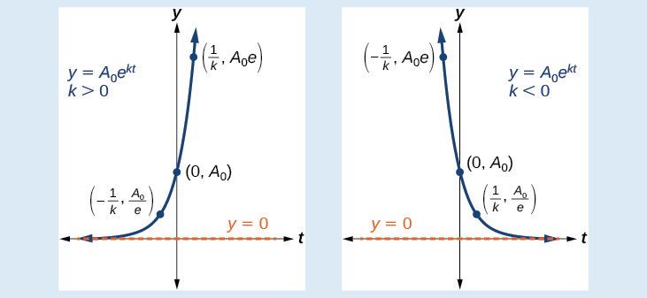$Two graphs of y=(A_0)(e^(kt)) with the asymptote at y=0. The first graph is of when k>0 and with the labeled points (1/k, (A_0)e), (0, A_0), and (-1/k, (A_0)/e). The second graph is of when k<0 and with the labeled points (-1/k, (A_0)e), (0, A_0), and (1/k, (A_0)/e).$ Figure $\PageIndex{5}$: Exponential Functions model
exponential growth ($k>0$) $\quad$ and $\quad$ exponential decay ($k<0$)

Exponential Growth

Example $\PageIndex{5}$: Find growth rate and model equation

A population of bacteria doubles every hour. If the culture started with $10$ bacteria, construct an equation that models the population as a function of time.

Solution

When an amount grows at a fixed percent per unit time, the growth is exponential. To find $A_0$ we use the fact that $A_0$ is the amount at time zero, so $A_0=10$. To find $k$, use the fact that after one hour $(t=1)$ the population doubles from $10$ to $20$.The formula is derived as follows

\[\begin{align*} y&=A_0e^{kt} &&\text{Formula}\\ 20&= 10e^{k\cdot 1}&&\text{Substitute given values}\\ 2&= e^k &&\text{Divide by 10}\\ \ln2&= k &&\text{Take the natural logarithm} \end{align*}\]

The growth rate is $k=\ln(2)$. $\ln(2) \approx 0.6931 $ so the equation could be written $y=10e^{0.6931t}$. However, a more exact version of the equation can be obtained by writing the equation in terms of $\color{Cerulean}{e^k}$, the growth factor. Using some log properties we get $y=10e^{(\ln2)t}=10{ ( {\color{Cerulean}{e^{\ln2}}} )}^t=10·{\color{Cerulean}{2}}^t$

Model Equations: using growth rate $k$ approximation: $y=10e^{0.6931t}$ or more exactly: $y=10·2^t$

Analysis. The population of bacteria after ten hours using $y=10·2^t$ is $10,240$. We could describe this amount is being of the order of magnitude $10^4$. The population of bacteria after twenty hours is $10,485,760$ which is of the order of magnitude $10^7$, so we could say that the population has increased by three orders of magnitude in ten hours.

A cautionary word about rounding. If the rounded approximation $k=0.6931$ had been used, the result would be $10,235$. If the full precision of your calculator is used to represent $k$ by using the [2nd][ANS] feature or [STO] and [MEMVAR] functions, for example, the result of $10,240$ would still be obtained. This illustrates that using rounded intermediate results produces rounding errors, so avoid getting answers that sometimes are significantly "off." Always use exact values or the full precision of your calculator in calculations to reduce or eliminate rounding errors.

Example $\PageIndex{6}$r: Find model equation, total amount and time, given a growth rate

It is estimated that the population of a certain small town is $93,000$ people with an annual growth rate of $2.6$%. If the population continues to increase exponentially at this rate:

Estimate the population in $7$ years' time.
Estimate the time it will take for the population to reach 120,000 people.

Solution

We begin by constructing a mathematical model based on the given information. Here the initial population $P_{0} = 93,000$ people and the growth rate $r = 2.6$% $= 0.026$. The following model gives population in terms of time measured in years:

\[ \begin{align}
A(t) &=A_0e^{kt} & &\text{Formula} \nonumber \\
P(t)&=93,000 e^{0.026 t} &&\text{Model equation} \label{ex5} \end{align} \]

a. Use this model equation (\ref{ex5}) to estimate the population in $t = 7$ years.

$\begin{aligned} P(t) &=93,000 e^{0006(\color{Cerulean}{7}\color{black}{)}} \\ &=93,000 e^{0.182} \\ & \approx 111,564 \quad people \end{aligned}$

b. Use this model equation (\ref{ex5}) to determine the time it takes to reach $P (t) = 120,000$ people.

$\begin{aligned} P(t) &=93,000 e^{0.026 t} \\ \color{Cerulean}{120,000} &\color{black}{=}93,000 e^{0.026 t} \\ \frac{120,000}{93,000} &=e^{0.026 t} \\ \frac{40}{31} &=e^{0.026 t} \end{aligned}$

Take the natural logarithm of both sides and then solve for $t$.

$\ln \left(\frac{40}{31}\right)=\ln e^{0.026 t}$
$\ln \left(\frac{40}{31}\right)=0.026 t \ln e$
$\ln \left(\frac{40}{31}\right)=0.026 t \cdot 1$
$\frac{\ln \left(\frac{40}{31}\right)}{0.026}=t$

Using a calculator,

$t=\ln (40 / 31) / 0.026 \approx 9.8\quad years$

Answer:

$111,564$ people
$9.8$ years

Often the growth rate $k$ is not given. In this case, we look for some other information so that we can determine it and then construct a mathematical model. The general steps are outlined in the following example.

Example $\PageIndex{7}$: Find growth rate, model equation, and total amount

Under optimal conditions Escherichia coli (E. coli) bacteria will grow exponentially with a doubling time of $20$ minutes. If $1,000$ E. coli cells are placed in a Petri dish and maintained under optimal conditions, how many E. coli cells will be present in $2$ hours?

Solution

The goal is to use the given information to construct a mathematical model based on the formula $A(t)=A_0e^{kt}$.

Step 1: Find the growth rate $k$. Use the fact that the initial amount, $A_{0} = 1,000$ cells, doubles in $20$ minutes. That is, $A(t) = 2,000$ cells when $t = 20$ minutes.

$\begin{aligned} A(t) &=A_{0} e^{k t} \\ \color{Cerulean}{2,000} &\color{black}{=}1,000 e^{k \color{Cerulean}{20}} \end{aligned}$

Solve for the only variable $k$.

$\begin{aligned} 2,000 &=1,000 e^{k 20} \\ \frac{2,000}{1,000} &=e^{k 20} \\ 2 &=e^{k 20} \\ \ln (2) &=\ln e^{k 20} \\ \ln (2) &=k 20 \ln e \\ \ln (2) &=k 20 \cdot 1 \\ \frac{\ln (2)}{20} &=k \end{aligned}$

Step 2: Write a mathematical model based on the given information for the number of E. coli cells in terms of time in minutes. Here $k ≈ 0.0347$, which is about $3.5$% growth rate per minute. So we could use the equation $ A(t)=1,000 e^{ 0.0347 t}$ for our model. However, we will use the exact value for $k$ in our model. This will allow us to avoid round-off error in the final result. Use $A_{0} = 1,000$ and $k=\ln (2) / 20$:

$\begin{aligned}
A(t)&=1,000 e^{ (\ln (2) / 20) t} \\
&=1,000 e^{\tfrac{\ln (2) }{20} t} \\
&=1,000 e^{\ln (2) \tfrac{t}{20} } \\
&=1,000 (e^{\ln (2)})^ {t/20 } \\
A(t)&=1,000 (2)^ {t/20 } && \text{Alternate form of Model equation}
\end{aligned}$

This equation models the number of E. coli cells in terms of time in minutes.

Step 3: Use the function to answer the questions. In this case, we are asked to find the number of cells present in $2$ hours. Because time is measured in minutes, use $t = 120$ minutes to calculate the number of E. coli cells.

$\begin{aligned} A( {\color{Cerulean}{120}} ) &=1,000 \cdot (2)^{ {\color{Cerulean}{120}} /20} \\ &=1,000 \cdot 2^{6} \\ &=64,000 \text { cells } \end{aligned}$

Answer:

In two hours $64,000$ cells will be present. (The answer obtained when $k= 0.0347$ is $64,328 $ cells.)

We can now solve applications that give us enough information to determine the rate of growth. We can then use that rate of growth to predict other situations.

Example $\PageIndex{8}$m: Find growth rate, model equation, and total amount

Researchers recorded that a certain bacteria population grew from $100$ to $300$ in $3$ hours. At this rate of growth, how many bacteria will there be $24$ hours from the start of the experiment?

Solution:

This problem requires two main steps. First we must find the unknown rate, $k$. Then we use that value of $k$ to help us find the unknown number of bacteria. Use the formula $A(t)=A_0e^{kt}$.

Step 1: Find the growth rate $k$. Identify values for the variables in the formula. $A =300$, $A_{0} =100$, $k =?$, $t =3$ hours.

$\begin{aligned} A(t) &=A_{0} e^{k t} &&\text{formula} \\
300&=100 e^{k \cdot 3} &&\text{substitute. only one variable left - solve for k} \\
3&=e^{3 k} \\
\ln 3&=\ln e^{3 k} &&\text{Take the natural log of each side.} \\
\ln 3&=3 k \ln e &&\text{Use the Power Property. } \\
\ln 3&=3 k \ln e &&\text{ } \\
\frac{\ln 3}{3}&=k &&\text{ln e = 1 } \\
k &\approx 0.366 \\
\end{aligned}$

Step 2: Write the model equation using $A_{0} =100$ and $k =\frac{\ln 3}{3} $. We use this revised equation to predict the number of bacteria $A(t)$ there will be in $t$ hours.

$A(t)=100 e^{\frac{\ln 3}{3} t} \qquad $ or $\qquad A(t)=100 e^{0.366 t} \qquad $ Model equations

Step 3: Use the function to answer the questions. How many bacteria will there be $t$ hours from the start of the experiment? Substitute in the value $t=24$ and evaluate.

$A(24)=100 e^{\frac{\ln 3}{3} \cdot 24}$
$A(24) = 656,100$

At this rate of growth, they can expect $656,100$ bacteria. (The answer obtained when $k= 0.366$ is $652,894 \;$ bacteria.)

Example $\PageIndex{9}$: Find model if not given initial amount

According to Moore’s Law, the doubling time for the number of transistors that can be put on a computer chip is approximately two years. Give a function that describes this behavior.

Solution

Start with the formula Use the formula $A(t)=A_0e^{kt}$.

Step 1. Find the growth rate $k$. Identify values for the variables in the formula. $A =2 A_{0}$, $k =?$, $t =2$ years.

$\begin{aligned} A(t) &=A_{0} e^{k t} &&\text{formula} \\
2 A_{0}&=A_{0} e^{k \cdot 2} \\
2&=e^{2 k} &&\text{DIvide both sides by }A_{0} \\
\ln 2&=\ln e^{2 k} &&\text{Take the natural log of each side.} \\
\ln 2&=2k \ln e &&\text{Use the Power Property. } \\
\frac{\ln 2}{2}&=k &&\text{ln e = 1 } \\
\end{aligned}$

The function is $A(t)=A_0e^{\tfrac{\ln2}{2}t}$ or $ A(t)=A_0(2)^{\ce{t/2}}$.

$try-it.png$ Try It $\PageIndex{9}$ma

Researchers recorded that a certain bacteria population grew from $100$ to $500$ in $6$ hours. At this rate of growth, how many bacteria will there be $24$ hours from the start of the experiment?
Recent data suggests that, as of 2013, the rate of growth predicted by Moore’s Law no longer holds. Growth has slowed to a doubling time of approximately three years. Find the new function that takes that longer doubling time into account.

a. Answer: There will be $62,500$ bacteria.

b. Answer: $f(t)=A_0e^{\tfrac{\ln2}{3}t}$ or $A(t)=A_0(2)^{t/3}$

Exponential Decay

When the growth rate is negative the function models exponential decay. With exponential decay, quantities are declining at a rapid rate. The rate of decay $k$, is directly proportional to the size of the quantity and is negative. The main example of exponential decay is radioactive decay. Radioactive elements and isotopes spontaneously emit subatomic particles, and this process gradually changes the substance into a different isotope. For example, the radioactive isotope Uranium-238 eventually decays into the stable isotope Lead-206. This is a random process for individual atoms, but overall the mass of the substance decreases according to the exponential decay formula. One of the common terms associated with exponential decay is half-life, the length of time it takes an exponentially decaying quantity to decrease to half its original amount. Every radioactive isotope has a half-life, and the process describing the exponential decay of an isotope is called radioactive decay.

Example $\PageIndex{10}$n: Exponential decay - find the equation

Suppose that a certain population of bacteria has an annual decay rate of 10%. Starting with 20,000 bacteria, how many bacteria will be left in 3 years?

Solution

Start with the formula $A(t)=A_0e^{kt}$.

Identify values for the variables in the formula. $A =?$, $ A_{0}=20,000$, $k =10 \% \text{ decay } \longrightarrow k=-0.10$, $t =3$ years.

$\begin{aligned} A(t) &=A_{0} e^{k t} &&\text{formula} \\
A(3)&=20000 e^{-0.10 \cdot 3} \\
A(3)&\approx 148.1636 &&\text{grams} \\
\end{aligned}$

Example $\PageIndex{11}$c: Exponential decay - find the equation and original amount

The loudness of a sound dies down at an exponential rate of 6.91. If it takes .2 seconds for a loud clap of thunder to diminish to the sound level of a whisper (of 30 decibels), how loud was the clap of thunder originally?

Solution

Start with the formula $A(t)=A_0e^{kt}$.

Identify values for the variables in the formula. $A =30$, $ A_{0}=? $, $|k| = 6.91 \text{ decay } \longrightarrow k=-6.91$, $t =.2$ seconds.

$\begin{aligned} A(t) &=A_{0} e^{k t} &&\text{formula} \\
30&=A_{0} e^{-6.91 \cdot .2} \\
30e^{6.91 \cdot .2} &=A_{0} \\
&=A_{0} \approx 119.5 &&\text{decibels} \\
\end{aligned}$

Example $\PageIndex{12}$c: Exponential decay - find the equation and elapsed time

A lawmaker once introduced legislation that would force Americans to cut back on their consumption of salt. It never passed the House, but it proposed that each year restaurants would be mandated to decrease sodium levels by two and a half percent annually. If all restaurants started out using a collective total of 5,000 kilograms of salt initially annually, and they were asked to reduce their consumption by two and a half percent each year, how long would it take to reduce their collective consumption to 3000 kg per year?

Start with the formula $A(t)=A_0e^{kt}$.

Identify values for the variables in the formula. $A =3000$, $ A_{0}=5000 $, $k = 2.5 \% \text{ decrease } \longrightarrow k=-.025$, $t =?$ seconds.

$\begin{aligned} A(t) &=A_{0} e^{k t} &&\text{Formula} \\
3000&=5000 e^{-.025 t} &&\text{Substitute values. Now solve for t} \\
\frac {3000}{5000}&=e^{-.025 t} \\
\ln(.6) &=\ln (e^{-.025 t}) &&\text{Take \( \ln $ of both sides} \\
\ln(.6) &=-.025 t \ln (e) &&\text{Power rule} \\
\ln(.6) &=-.025 t && \ln(e)=1 \\
t &=\dfrac{\ln(.6)}{-.025 } \\
t &\approx 20.4 &&\text{years} \\
\end{aligned}\)

Half-Life

Radioactive substances decay or decompose according to the exponential decay formula. The amount of time it takes for the substance to decay to half of its original amount is called the half-life of the substance. As with exponential growth processes that have a fixed doubling time. Similarly, exponential decay processes have a fixed half-life, the time in which one-half the original amount decays.

Example $\PageIndex{13}$: Radioactive Decay (half life) - find decay rate and equation

The half-life of carbon-14 is $5,730$ years. Express the amount of carbon-14 remaining as a function of time, $t$.

Solution

Start with the formula $A(t)=A_0e^{kt}$.

Identify values for the variables in the formula. $A =\frac{1}{2}A_{0}$, $ A_{0}=? $, $k = ?$, $t =5730$ years.

\[\begin{align*} A&= A_0e^{kt} \qquad &&\text{The continuous growth formula}\\
0.5A_0&= A_0e^{k\cdot 5730} \qquad &&\text{Substitute the half-life for t and } 0.5A_0 \text{ for } f(t)\\
0.5&= e^{5730k} &&\qquad \text{Divide by } A_0\\
\ln(0.5)&= 5730k \qquad &&\text{Take the natural log of both sides}\\
k&= \dfrac{\ln(0.5)}{5730} \qquad &&\text{Divide by the coefficient of k}\\
k & \approx −1.2097×10^{−4} \end{align*}\]

The function that describes this continuous decay is $A(t)=A_0e^{\left (\tfrac{\ln(0.5)}{5730} \right )t}$. We observe that $k$ is negative, as expected in the case of exponential decay. Other forms of this function include $A(t)=A_0e^{.00012t}$ and $A(t)=A_0\left (\tfrac{1}{2} \right )^{t/5730} $

Example $\PageIndex{14}$m: Exponential Decay - find decay rate, equation, amount remaining

The half-life of radium-226 is $1,590$ years. How much of a $100$ mg sample will be left in $500$ years?

Solution:

Start with the formula $A(t)=A_0e^{kt}$. Identify values for the variables in the formula.

Step 1. Identify values of the variables needed to find the decay constant $k$: At time t=1590 years, $A(1590) =\frac{1}{2}A_{0}$, $ A_{0}=?$, $k = ?$, $t =1590$ years. Since the next part of the question asks how much of a $100$ mg sample will be left in $500$ years, we may also choose to use $A(1590) =50$ mg, and $ A_{0}=100$ mg instead.

\[\begin{align*} A(t)&= A_0e^{kt} &&\text{The continuous growth formula}\\
50&=100 e^{k \cdot 1590} &&\text{Substitute values. Now solve for k} \\
0.5&=e^{1590 k} &&\text{ } \\
\ln 0.5&=\ln e^{1590 k} &&\text{Take the natural log of each side. } \\
\ln 0.5&=1590 k \ln e &&\text{Use the Power Property. } \\
\ \ln 0.5&=1590 k && \ln(e)=1 \\
k &=\frac{\ln 0.5}{1590} &&\text{exact answer} \\
k &\approx -.00044 &&\text{approximate answer} \end{align*}\]

Step 2: Write the model equation that predicts the amount of radium-226 $A(t)$ there will be left in $t$ years. The decay factor is $e^k = e^{\ce(\ln 0.5)/1590}} = (e^{\ln 0.5})^{\ce{1/1590}} =(.5) ^ {\frac{1}{1590}}$. Also $e^{kt} = (e^k)^t$

$A(t)= 100 (.5)^{ t/1590 } \qquad$ or $ \qquad A(t) \approx 100 \: e^{-.00044t} \qquad $ Model Equations

Step 3: Use the model equation to answer the question. How much of a $100$ mg sample will be left in $500$ years? Here the values of the variables are $A(500) =?$ mg and $t =500$ years.

\[\begin{align*}
A(500) &=100 (.5)^{ 500/1590} \\
& \approx 80.41 \end{align*}\]

In $500$ years there would be approximately $80.4$ mg remaining. (The answer obtained when $k=-.00044$ is $80.3 $ mg.)

Example $\PageIndex{15}$r: Exponential Decay - find decay rate, model equation, and elapsed time

Due to radioactive decay, caesium-137 has a half-life of $30$ years. How long will it take a $50$-milligram sample to decay to $10$ milligrams?

Solution:

Start with the formula $A(t)=A_0e^{kt}$. Identify values for the variables in the formula.

Step 1: Find the growth rate $k$. Identify values for the variables in the formula: $A(30) =25$ mg, $ A_{0}=50$ mg, $k = ?$, $t =30$ years.

$\begin{aligned}
A(t)&=A_0e^{kt} \\
25&=50 e^{k \cdot 30} \\
\frac{25}{50}&=e^{30 k} \\
\ln \left(\frac{1}{2}\right)&=\ln e^{30 k} \\
\ln (.5) &=30 k \ln e &&\color{Cerulean} { \text{Recall that }\ln e=1. }\\
k &=\frac{\ln (.5)}{30} \\
k &\approx -0.0231049 \end{aligned}$

Step 2: Write the model equation to predict the amount of caesium-137 that will be left in a $50$-milligram sample after $t$ years. Note that $k \approx-0.0231$ is negative. However, we will use the exact value to construct a model that gives the amount of cesium-137 with respect to time in years.

$\begin{aligned}
A(t)&=50 e^{(ln (.5) / 30) t}\\
&=50 e^{ln (.5) t/30}\\
&=50 \left( e^{(ln (.5)} \right)^{ t/30} &&\color{Cerulean} { \text{Use the Inverse Property }e^{\ln M}=M. } \\
A(t)&=50 (.5)^{ t/30} &&\text{or alternatively } A(t)=50e^{-0.0231t} \text{ Model equations}
\end{aligned}$

Step 3: Use the model to find $t$ when $A (t) = 10$ milligrams.

$\begin{aligned}10&=50 (.5)^ {t/30} \\
\frac{10}{50}&=(.5)^{t/30} \\
\ln (.2) &=\ln (.5)^{t/30}\\
\ln(.2)&=t/30 \ln (.5) \\
\ln(.2)&=\dfrac{\ln (.5)}{30} t\\
t &= \ln(.2) \cdot \dfrac {30}{\ln (.5)}\\
t &=\frac{30 \ln(.2)}{\ln .5} \\
t &\approx 69.66 \end{aligned}$

Answer: It will take $t ≈ 69.66$ years to decay to $10$ milligrams. (The answer obtained when $k=-0.0231$ is $t ≈ 69.67.)$

Radiocarbon Dating

The formula for radioactive decay is important in radiocarbon dating, which is used to calculate the approximate date a plant or animal died. Radiocarbon dating was discovered in 1949 by Willard Libby, who won a Nobel Prize for his discovery. It compares the difference between the ratio of two isotopes of carbon in an organic artifact or fossil to the ratio of those two isotopes in the air. It is believed to be accurate to within about $1\%$ error for plants or animals that died within the last $60,000$ years. As long as a plant or animal is alive, the ratio of the two isotopes of carbon in its body is close to the ratio in the atmosphere. When it dies, the carbon-14 in its body decays and is not replaced. By comparing the ratio of carbon-14 to carbon-12 in a decaying sample to the known ratio in the atmosphere, the date the plant or animal died can be approximated. While the carbon-14 technique only works on plants and animals, there are other similar dating techniques, using other radioactive isotopes, that are used to date rocks and other inorganic matter.

Example $\PageIndex{16}$r: Carbon dating - find decay rate, model equation, and elapsed time

An ancient bone tool is found to contain $25$% of the carbon-14 normally found in bone. Given that carbon-14 has a half-life of $5,730$ years, estimate the age of the tool.

Solution

Start with the formula $A(t)=A_0e^{kt}$. Identify values for the variables in the formula.

Step 1: Find the growth rate $k$. Identify values for the variables in the formula: $A(5,730) =\frac{1}{2}A_0$ mg, $ A_{0}=?$ mg, $k = ?$, $t =5,730$ years. Notice below that when both sides are divided by $A_{0}$, the remaining exponential equation is only in terms of $k$. This shows that half-life is independent of the initial amount.

$\begin{aligned}
A(t)&=A_0e^{kt} \\
\frac{1}{2} A_{0}&=A_{0} e^{k 5,730} \\
.5 &=e^{k5,730} \\
\ln (.5) &=\ln e^{k 5,730} \\
\ln (.5) &= 5,730k\ln e \\
k &= \frac{\ln (.5) }{5,730} \\
k &\approx -.00012
\end{aligned}$

Step 2: Write the model equation that predicts the amount of carbon-14 remaining in the bone $t$ years after death of the object.

$
A(t) =A_0e^{-.00012t} \qquad \text{or} \qquad
A(t) =A_{0} e^{ \frac{\ln (.5) }{5,730} t} =A_{0} \left( e^{\ln (.5) }\right) ^\frac {t}{5,730} =A_{0} \: (.5)^{t/5730} \quad \text{ Model equations}
$

Step 3: Use the model to find the time $t$ it takes the carbon-14 to decay to $25$% of the initial amount, or $A (t) = 0.25A_{0}$

$\begin{aligned}
A(t)&=A_{0} \: (.5)^{t/5730} \\
0.25A_{0} &=A_{0} (.5)^ {t/5730} \\
0.25 &=(.5)^ {t/5730} \\
\ln (0.25) &=\ln (.5)^ {t/5730} \\
\ln (0.25) &=t/5730 \: ( \ln (.5)) \\
t &= \frac{5,730 \ln (0.25)}{\ln (.5)} \\
t &\approx 11,460\end{aligned}$

Answer: The tool is approximately $11,460\;$ years old. (The answer obtained when $k=-.00012$ is $11,552 $ years old).

$try-it.png$ Try It $\PageIndex{16a}$A

a. Researchers recorded that a certain bacteria population declined from $700,000$ to $400,000$ in $5$ hours after the administration of medication. At this rate of decay, how many bacteria will there be $24$ hours from the start of the experiment?

b. The half-life of plutonium-244 is $80,000,000$ years. Find function gives the amount of carbon-14 remaining as a function of time, measured in years.

a. Answer: There will be $47,699$ bacteria.
( $k=\frac{1}{5} \ln ( \frac{4}{7} ) \approx -.11192 $ )

b. Answer: $f(t)=A_0e^{−0.0000000087t}$
( $ k = \frac{1}{8} \ln (.5) \times 10^{-7} $ )

$try-it.png$ Try It $\PageIndex{16b}$m

a. The half-life of strontium-90 is about $28$ years. How long will it take a $36$ milligram sample of strontium-90 to decay to $30$ milligrams?

b. Cesium-137 has a half-life of about $30$ years. If we begin with $200$ mg of cesium-137, how long will it take until only $1$ milligram remains?

c. The half-life of magnesium-27 is $9.45$ minutes. How much of a $10$-mg sample will be left in $6$ minutes?

d. The half-life of radioactive iodine is $60$ days. How much of a $50$-mg sample will be left in $40$ days?

a .Answer: $7.4$ years

b .Answer: $229.3$ years

c .Answer: There will be $6.43$ mg left.

d .Answer: There will be $31.5$ mg left.

Newton’s Law of Cooling

Exponential decay can also be applied to temperature. When a hot object is put into a place that is at a lower temperature, the object’s temperature will decrease exponentially, leveling off as it approaches the surrounding air temperature.

NEWTON’S LAW OF COOLING

The temperature of an object, $T$, in surrounding air with temperature $S$ will behave according to the formula

$T(t)=Ae^{kt}+S \quad
\begin{cases}
t \;\;\text{ is time}\\
A \;\;\text{ is the difference between the initial temperature of the object and the surroundings} \\
k \;\;\text{ is a constant, the continuous rate of cooling of the object }\\
\end{cases}
$

Example $\PageIndex{17}$: Using Newton’s Law of Cooling

A cheesecake is taken out of the oven with an ideal internal temperature of $165°F$, and is placed into a $35°F$ refrigerator. After $10$ minutes, the cheesecake has cooled to $150°F$. If we must wait until the cheesecake has cooled to $70°F$ before we eat it, how long will we have to wait?

Solution

Because the surrounding air temperature in the refrigerator is $35$ degrees, the cheesecake’s temperature will decay exponentially toward $35$, following the equation

$T(t)=Ae^{kt}+35$

Step 1. Find $A$. We know the initial temperature was $165$, so $T(0)=165$.

\[\begin{align*} 165&= Ae^{k0}+35 &&\text{Substitute } (0,165)\\
165&= A+35 \\
A&= 130 &&\text{Solve for A}
\end{align*}\]

At the conclusion of this step, we now have a modifed formula, $T(t)=130e^{kt}+35$

Step 2. Find $k$. To do this, use our modified formula, $T(t)=130e^{kt}+35$, and the fact that $T(10)=150$.

\[\begin{align*}
T(t)&=130e^{kt}+35 \\
150&= 130e^{k10}+35 \qquad &&\text{Substitute } (10, 150)\\
115&= 130e^{k10} \qquad &&\text{Subtract 35}\\
\dfrac{115}{130}&= e^{10k} \qquad &&\text{Divide by 130}\\
\ln\left (\dfrac{115}{130} \right )&= 10k \qquad &&\text{Take the natural log of both sides}\\
k&= \dfrac{\ln \left (\dfrac{115}{130} \right )}{10}\\
&= -0.0123 \qquad &&\text{Divide by the coefficient of k} \end{align*}\]

At the end of this step we now have the equation for the cooling of the cheesecake: $T(t)=130e^{–0.0123t}+35$.

Another form this equation can take is $T(t)=130e^{\frac{\ln \left( \tfrac{115}{130} \right) }{10}}+35$ which simplifies to $T(t)=130 \left( \frac{115}{130} \right )^\tfrac{t}{10}+35$.

Step 3. Now we can solve for the time it will take for the temperature to cool to $70$ degrees.

\[\begin{align*} 70&= 130e^{-0.0123t}+35 \qquad \text{Substitute in 70 for } T(t)\\ 35&= 130e^{-0.0123t} \qquad \text{Subtract 35}\\ \dfrac{35}{130}&= e^{-0.0123t} \qquad \text{Divide by 130}\\ \ln \left (\dfrac{35}{130} \right )&= -0.0123t \qquad \text{Take the natural log of both sides}\\ t&= \dfrac{\ln \left (\dfrac{35}{130} \right )}{-0.0123}\\ &\approx 106.68 \qquad \text{Divide by the coefficient of t} \end{align*}\]

It will take about $107$ minutes, or one hour and $47$ minutes, for the cheesecake to cool to $70°F$. (The answer, rounded to the nearest minute, obtained when $k=\frac{\ln \left (\tfrac{115}{130} \right ) $ is the same).

$try-it.png$ Try It $\PageIndex{17}$

A pitcher of water at $40$ degrees Fahrenheit is placed into a $70$ degree room. One hour later, the temperature has risen to $45$ degrees. How long will it take for the temperature to rise to $60$ degrees?

Answer: $6.026$ hours

Logistic Growth Models

Exponential growth cannot continue forever. Exponential models, while they may be useful in the short term, tend to fall apart the longer they continue. Consider an aspiring writer who writes a single line on day one and plans to double the number of lines she writes each day for a month. By the end of the month, she must write over $17$ billion lines, or one-half-billion pages. It is impractical, if not impossible, for anyone to write that much in such a short period of time. Eventually, an exponential model must begin to approach some limiting value, and then the growth is forced to slow. For this reason, it is often better to use a model with an upper bound instead of an exponential growth model, though the exponential growth model is still useful over a short term, before approaching the limiting value.

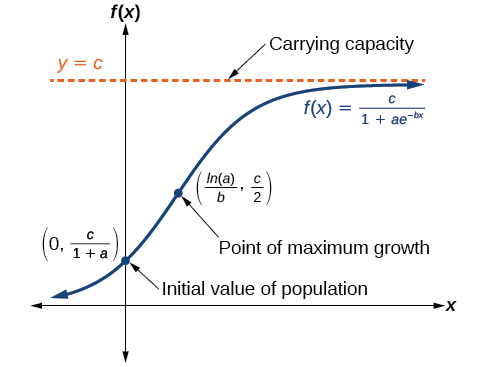
The logistic growth model is approximately exponential at first, but it has a reduced rate of growth as the output approaches the model’s upper bound, called the carrying capacity. For constants $a$, $b$, and $c$, the logistic growth of a population over time $x$ is represented by the model

$f(x)=\dfrac{c}{1+ae^{−bx}}$

The graph in Figure $\PageIndex{6}$ shows how the growth rate changes over time. The graph increases from left to right, but the growth rate only increases until it reaches its point of maximum growth rate, at which point the rate of increase decreases.

LOGISTIC GROWTH

The logistic growth model is

\[f(x)=\dfrac{c}{1+ae^{−bx}}\]

where

$\dfrac{c}{1+a}$ is the initial value, $f(0)$
$c$ is the carrying capacity, or limiting value, $f(\infty )$
$b$ is a constant determined by the rate of growth.

$Graph of f(x)=c/(1+ae^(-tx)). The carrying capacity is the asymptote at y=c. The initial value of population is (0, c/(1+a)). The point of maximum growth is (ln(a)/b, c/2).$
Figure $\PageIndex{6}$

Example $\PageIndex{18}$: Using the Logistic-Growth Model

An influenza epidemic spreads through a population rapidly, at a rate that depends on two factors: The more people who have the flu, the more rapidly it spreads, and also the more uninfected people there are, the more rapidly it spreads. These two factors make the logistic model a good one to study the spread of communicable diseases. And, clearly, there is a maximum value for the number of people infected: the entire population.

For example, at time $t=0$ there is one person in a community of $1,000$ people who has the flu. So, in that community, at most $1,000$ people can have the flu. Researchers find that for this particular strain of the flu, the logistic growth constant is $b=0.6030$. Estimate the number of people in this community who will have had this flu after ten days. Predict how many people in this community will have had this flu after a long period of time has passed.

Solution

We substitute the given data into the logistic growth model $f(x)=\dfrac{c}{1+ae^{−bx}}$

Step 1. Find one of the constants by evaluating $f$ when $x \rightarrow \infty $. This results in $e^{-bx}$ approaching zero, so $f(x \rightarrow \infty) = c$. Because at most the entire population of the community, $1,000$ people, can eventually get the flu, we know the limiting value is $c=1000$.

Step 2. Find one of the constants by evaluating $f$ when $x=0$. We are given $f(0) = 1$. Therefore $\dfrac{c}{1+a}=1$, from which it follows that $a=999$.

Step 3. Given that the logistic growth constant is $b=0.6030$, we obtain the model equation $f(x)=\dfrac{1000}{1+999e^{−0.6030x}}$.

Step 4. Use the model. This model predicts that, after ten days, the number of people who have had the flu is $f(10)=\dfrac{1000}{1+999e^{−0.6030\cdot 10}}≈293.8$. Because the actual number must be a whole number (a person has either had the flu or not) we round to $294$. In the long term, the number of people who will contract the flu is the limiting value, $c=1000$.

$Graph of f(x)=1000/(1+999e^(-0.5030x)) with the y-axis labeled as “Cases” and the x-axis labeled as “Days”. There was 1 case on day 0, 20 on day 5, 294 on day 10, and 1000 on day 21.$

Figure $\PageIndex{7}$: The graph of $f(x)=\dfrac{1000}{1+999e^{−0.6030x}}$

After a long time has passed, the entire community of 1000 people will have had this flu.

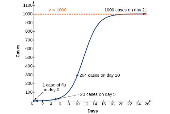
Analysis. Remember that, because we are dealing with a virus, we cannot predict with certainty the number of people infected. The model only approximates the number of people infected and will not give us exact or actual values. The graph in Figure $\PageIndex{7}$ gives a good picture of how this model fits the data.

$try-it.png$ Try It $\PageIndex{18}$

Using the model in the Example above, estimate the number of cases of flu on day $15$.

Answer: $895 \;$ cases on day $15$

Key Concepts

The basic exponential function is $f(x)=ab^x$. If $b>1$, we have exponential growth; if $0<b<1$, we have exponential decay.
We can also write this formula in terms of continuous growth as $A=A_0e^{kx},$ where $A_0$ is the starting value. If $A_0$ is positive, then we have exponential growth when $k>0$ and exponential decay when $k<0$.
In general, we solve problems involving exponential growth or decay in two steps. First, we set up a model and use the model to find the parameters. Then we use the formula with these parameters to predict growth and decay.
We can find the age of an organic artifact by measuring the amount of carbon-14 (which is subject to exponential decay) remaining in the artifact.
Given a substance’s doubling time or half-time, we can find a function that represents its exponential growth or decay.
We can use Newton’s Law of Cooling to find how long it will take for a cooling object to reach a desired temperature, or to find what temperature an object will be after a given time.
We can use logistic growth functions to model real-world situations where the rate of growth changes over time, such as population growth, spread of disease, and spread of rumors.
Any exponential function with the form $y=A_0b^x$ can be rewritten as an equivalent exponential function with the form $y=A_0e^{kx}$ where $k=\ln b$.

Jay Abramson (Arizona State University) with contributing authors. Textbook content produced by OpenStax College is licensed under a Creative Commons Attribution License 4.0 license. Download for free at https://openstax.org/details/books/precalculus.